


81:22 |
Cleve Moler and Jack Little |
Fig. 12. A two-dimensional plot produced by contemporary MATLAB.
4 EVOLUTION OF MATLAB
While preserving its roots in matrix mathematics, MATLAB has continued to evolve to meet the changing needs of engineers and scientists. Here are some of the key developments [na Moler 2018c; na Moler 2018d].
4.1 Data Types
By 1992 MathWorks had over 100 staff members and by 1995, over 200. About half of them had degrees in science and engineering and worked on the development of MATLAB and its various toolboxes. As a group, they represented a large and experienced collection of MATLAB programmers. Suggestions for enhancements to the language often come from these users within the company itself.
MATLAB was being used for the design and modeling of embedded systems, which are controllers with specific real-time functions within larger electrical or mechanical systems. Such controllers often have only single precision floating point or fixed-point arithmetic. The designers of embedded systems desired the ability develop their algorithms using the native arithmetic of the target processors. This motivated the introduction of several new data types into MATLAB, but without the use of actual type declarations.
Proc. ACM Program. Lang., Vol. 4, No. HOPL, Article 81. Publication date: June 2020.

A History of MATLAB |
81:23 |
Fig. 13. A three-dimensional plot produced by contemporary MATLAB.
For many years MATLAB had only one numeric data type, IEEE standard 754 double precision floating point, stored in the 64-bit format.
format long
phi = (1 + sqrt(5))/2
phi = 1.618033988749895
Support for numeric data types other than double was gradually added to MATLAB between 1996 and 2004. Requiring only 32 bits of storage, single precision floating point cuts memory requirements for large arrays in half. It may or may not be faster.
MATLAB does not have declarations, so single precision variables are obtained from double precision ones by an executable conversion function.
p = single(phi)
p=
single 1.6180340
Proc. ACM Program. Lang., Vol. 4, No. HOPL, Article 81. Publication date: June 2020.
81:24 |
Cleve Moler and Jack Little |
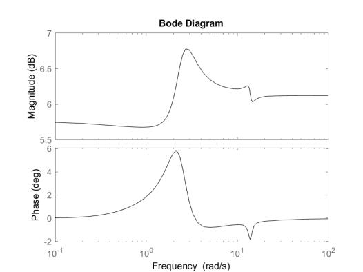
Fig. 14. A Bode plot from Control Systems Toolbox shows the magnitude and phase shift of the frequency response of a system.
Unsigned integer types uint8 and uint16 were initially used just for storage of images; no arithmetic was required.
In 2004 MATLAB 7 introduced full arithmetic support for single precision, four unsigned integer data types (uint8, uint16, uint32, and uint64) and four signed integer data types (int8, int16, int32, and int64). MATLAB 7 also introduced the new logical type.
q = uint16(1000*phi) r = int8(-10*phi)
s = logical(phi)
q=
uint16
1618
r=
int8 -16
s=
logical 1
Proc. ACM Program. Lang., Vol. 4, No. HOPL, Article 81. Publication date: June 2020.

The classic MATLAB interpreter counted every floating point operation, and reported the count if a statement is terminated with an extra comma. This feature is not available in today's MATLAB where the inner loops of matrix and other computations must be as efficient as possible. Here is a demonstration of the fact that inverting an n-by-n matrix requires slightly more than n^3 floating-poi ops.
A History
Fig. 15. Demonstration of the use of an extra comma to print the flops count in Classic MATLAB.
Published with MATLAB® R2019b
Let’s see how much storage is required for these variables:
Name |
Size |
Bytes |
Class |
p |
1x1 |
4 |
single |
phi |
1x1 |
8 |
double |
q |
1x1 |
2 |
uint16 |
r |
1x1 |
1 |
int8 |
s |
1x1 |
1 |
logical |
4.2 Sparse Matrices
In the folklore of matrix computation, it is said that J. H. Wilkinson defined a sparse matrix as any
matrix with enough zeros that it pays to take advantage of them. (He may well have said exactly this to his students, but it ought to be compared with this passage he wrote in the Handbook for Automatic Computation:
iv) The matrix may be sparse, either with the non-zero elements concentrated on a narrow
file:///C:/Users/moler/Documthents/Desktop/HOPL_xmas/html/flops.html
band centered on diagonal or alternatively they may be distributed in a less systematic manner. We shall refer to such a matrix as dense if the percentage of zero elements or its distribution is such as to make it uneconomic to take advantage of their presence.
[Wilkinson and Reinsch 1971, page 191].)
Iain Duff is a British mathematician and computer scientist known for his work on algorithms and software for sparse matrix computation. In 1990, he visited Stanford and gave a talk in the numerical analysis seminar. Moler attended the talk. So did John Gilbert, who was then at Xerox Palo Alto Research Center, and Rob Schreiber, from Hewlett Packard Research. They went to lunch
Proc. ACM Program. Lang., Vol. 4, No. HOPL, Article 81. Publication date: June 2020.
81:26 |
Cleve Moler and Jack Little |
at Stanford’s Tresidder Union and there Gilbert, Schreiber and Moler decided it was about time for MATLAB to support sparse matrices.
MATLAB 4 introduced sparse matrices in 1992 [Gilbert et al. 1992]. A number of design options
and design principles were explored. It was important to draw a clear distinction between the value of a matrix and any specific representation that might be used for that matrix [Gilbert et al. 1992,
page 4]:
We wish to emphasize the distinction between a matrix and what we call its storage class. A given matrix can conceivably be stored in many different ways—fixed point or floating point, by rows or by columns, real or complex, full or sparse—but all the different ways represent the same matrix. We now have two matrix storage classes in MATLAB, full and sparse.
Four important design principles emerged.
•The value of the result of an operation should not depend on the storage class of the operands, although the storage class of the result may. [Gilbert et al. 1992, page 10]
•No sparse matrices should be created without some overt direction from the user. Thus, the changes to MATLAB would not affect the user who has no need for sparsity. Operations on full matrices continue to produce full matrices.
•Once initiated, sparsity propagates. Operations on sparse matrices produce sparse matrices. And an operation on a mixture of sparse and full matrices produces a sparse result unless the operator ordinarily destroys sparsity. [Gilbert et al. 1992, page 5]
•The computer time required for a sparse matrix operation should be proportional to the number of arithmetic operations on nonzero quantities. [Gilbert et al. 1992, page 3]
(Some of these principles were rediscovered later in the design effort to add arithmetic support for single precision and the integer types.)
Only the nonzero elements of sparse matrices are stored, along with row indices and pointers to the starts of columns. The only change to the outward appearance of MATLAB was a pair of functions, sparse and full, to allow the user to provide a matrix and obtain a copy that has the specified storage class. Nearly all other operations apply equally to full or sparse matrices. The sparse storage scheme represents a matrix in space proportional to the number of nonzero entries, and most of the operations compute sparse results in time proportional to the number of arithmetic operations on nonzero entries. In addition, sparse matrices are printed in a different format that presents only the nonzero entries.
As an example, consider the classic finite difference approximation to the Laplacian differential operator. The function numgrid numbers the points in a two-dimensional grid, in this case -by- points in the interior of a square.
n = 100;
S = numgrid('S',n+2);
The function delsq creates the five-point discrete Laplacian, stored as a sparse -by- matrix, where = 2. With five or fewer nonzeros per row, the total number of nonzeros is a little less than 5 .
A = delsq(S); nz = nnz(A)
nz = 49600
Proc. ACM Program. Lang., Vol. 4, No. HOPL, Article 81. Publication date: June 2020.