194	7 Forces in Two and Three Dimensions

7.4.1 Example: Path Through a Tornado

You are part of a tornado-chaser team—a group of scientists trying to discover the inner workings of tornadoes. An important part of this work is to develop methods to measure the pressure and wind velocity inside the tornado. Your plan is to use many tiny projectiles with small accelerometers inside. You plan to shoot the projectiles through the tornado, pick them up afterwards, and read the recorded accelerations. Here, we will assume that the accelerometers record the acceleration in the x , y, and z-direction during flight. Here, we will develop a model for the flight of the projectile, and calculate realistic trajectories in order to learn how to launch the projectiles.

Sketch and Identify: Our task is to determine the motion of a projectile, characterized by its position r(t ). For the calculations, we use a coordinate system with the origin in the center of the tornado at ground level. The z-axis points in the vertical direction, with the positive direction upwards. We will launch the projectile from the position r(t0) = r0 with an initial velocity, v(t0) = v0 at t0 = 0.0 s.

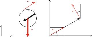
Model: While the projectile is in the air, the only contact force affecting the object is the force from the surrounding air, FD , in addition to gravity, G, as illustrated in Fig. 7.6.

Since the projectile will be moving fast, we use the square-law force model for the air resistance. However, in this case it is important to realize that the force depends on the velocity of the projectile, v, relative to the velocity of the wind, u(r). The square-law force model is therefore:

FD = −D (v − u) |v − u| ,

(7.30)

where for a spherical object we have that the prefactor is D 3.0ρd2, where d is the diameter of the sphere and ρ is the density of the surrounding air. Here, we will assume that the density of the surrounding air does not change significantly, and we

(A)	(B) y	-sin(	θ	)= - ry / r
v
FD				cos(θ)= rx / r
		uθ
y	cos(θ)= rx / r
G	ur	sin(θ)= ry / r
x				x

Fig. 7.6 a Free-body diagram of the projectile. b Illustration of the tangential direction in the tornado

7.4 Force Model—Viscous Force

195

will use ρ = 1.293 k/m3. Let us also assume that the projectile has a diameter of d = 0.02 m, and that its mass is m = 0.1 kg.

The force from gravity is G = −mg k, where k is the unit vector in the z-direction.

Newton’s second law: Newton’s second law gives the acceleration of the projectile:

ma = F j = FD + G .			(7.31)
		j
The acceleration is therefore:
a = −	D	(v − u) |v − u| − g k .	(7.32)
	m

and the initial conditions are r(t0) = r0 and v(t0) = v0.

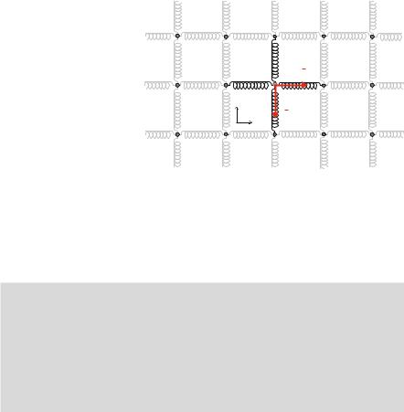
Model of wind velocity: However, in order to test and analyze the path of the projectile, we need a model for the velocity u in the tornado. Since we do not know this velocity-field, we will here use a model for the velocity taken from an analoguous situation. We can make an experimental tornado by rotating a thin cylinder in a fluid. For this case, we know that the velocity in the fluid will have the form:

u(r) = u(r )uˆθ ,

(7.33)

where the center of the cylinder is at the origin, and the speed, u(r ), depends only on the distance to the center of the cylinder, and the unit vector uˆθ points in the tangential direction, as illustrated in Fig. 7.6. The speed u(r ) has the following form:

u0	(r /r ) for r > r
u(r ) = u0	(r/r ) for r < r	,	(7.34)

where r is the radius of the cylinder.

We use this as a model for the velocity field inside the tornado to estimate the path of the projectile. Let us assume that we study a tornado with a radius of r = 10 m, and with a maximum wind speed of u0 = 50.0 m/s, which corresponds to a category F1 tornado.

Numerical solution: We can now use our theoretical model to find the motion of the projectile. We use a Euler-Cromer method to find the velocity and position vectors as function of time, starting from t = t0, and continuing until the projectile hits the ground.

Euler-Cromer’s method consists of the following steps:

v(t0 +	t ) v(t0) +	t a(t0, r(t0), v(t0))	(7.35)
r(t0 +	t ) r(t0) +	t v(t0 + t ) .	(7.36)

196	7 Forces in Two and Three Dimensions

This method is implemented in the following program:

from pylab import * m = 0.2

diam = 0.025 rho = 1.293

D = 3.0*rho*diam**2 Dm = D/m

g = array([0.0,0.0,9.8]) u0 = 50.0

rast = 5.0

r0 = array([-100.0,0.0,0.0]) alpha = 45.0*pi/180.0;

v0 = 100.0*array([cos(alpha),0,sin(alpha)]) time = 10.0

dt = 0.001

n = int(round(time/dt)) r = zeros((n,3),float) v = zeros((n,3),float) a = zeros((n,3),float) t = zeros(n,float)

r[0] = r0 v[0] = v0 i = 1

while (r[i,2]>=0.0) and (i<n): rr = norm(r[i])

if (rr>rast):

U = u0*(rast/rr) else:

U = u0*rr/rast

u = U*array([-r[i,1]/rr,r[i,0]/rr,0.0]) vrel = v[i] - u

aa = -g - Dm*norm(vrel)*vrel a[i] = aa

v[i+1] = v[i] + dt*aa r[i+1] = r[i] + dt*v[i+1] t[i+1] = t[i] + dt

i = i + 1 imax = i

ii = r_[1:imax]

Notice how we have used that the tangential vector to a point at (x , y) points in the direction (−y/r, x /r ), where r 2 = x 2 + y2.

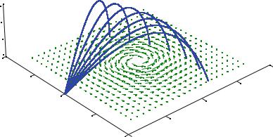
Analysis: We now have a tool to start addressing the motion of the projectile inside the tornado. Let us use this to test the path of a projectile launched from a distance of 100 m towards the center of the tornado with an initial speed v = 100 m/s.

Since the tornado is symmetric, we launch the projectile from the position r0 = −100 m i. We fire the projectile at an angle of 45◦ with the horizon, which corresponds to an angle of π/4 in radians, since this gives the maximum length when there is no air-resistance. The initial velocity is therefore v0 = 100 m/s cos(π/4) i +100 m/s sin(π/4) j. The resulting path is shown in Fig. 7.7.

The trajectory is hardly affected by the tornado. How can we change the trajectory to make it more sensitive to the wind speed? We could shoot it at an angle with the center, and not directly towards the center. This is attempted by introducing the angle θ , which gives the deviation from the line straight into the center. The initial velocity is now.

7.4 Force Model—Viscous Force

197

Z [M]

60

40

20

0 100

100

50

50

0

Y [M]		0
	-50	X [M]
		-50
		-100 -100

Fig. 7.7 Simulated trajectories of projectiles launched at different angles. The velocity field of the tornado is illustrated by the arrows

v0 = v0 (cos α cos θ i + cos α sin θ j + sin α k) ,

(7.37)

Simulations for various values of θ are given in Fig. 7.7.

Notice the change in trajectories for the various angles. The next step would be to see how easy it would be to find the velocity field from these trajectories or from a set of trajectories, but we will not pursue this direction here. From our discussion you should be able to see how we can use this model to address how to launch the projectile.

Test your understanding: Based on this analysis, would you recommend launching the projectile by shooting it into the tornado, or by ejecting them vertically as the tornado is passing from a container ledged to the ground?

7.5 Force Model—Spring Force

When we introduced the spring model in one dimension, it was used to represent two different concepts:

•To model the force from a linearly elastic spring

•To represent the simplest position-dependent force model

Both of these interpretations are still important in twoand three-dimensional systems. We may use a spring model as a model for deformation, and we may use the spring model as a simplified model for a position-dependent force. However, we have more degrees of freedom, and we can therefore define a spring model in several different ways.

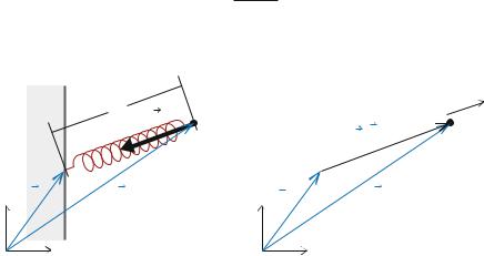
198	7 Forces in Two and Three Dimensions

Full Spring Model

Let us first see how the force due the deformation of a spring can be generalized in twoand three-dimensions. From one-dimensional experiments, we expect the force from a spring on the object attached to the spring to depend on the elongation of the spring and act in the direction of the spring. The situation is illustrated in Fig. 7.8. A spring is characterized by its equilibrium length, L0, and its spring constant, k. The force from the spring on the object is:

F = −k (L − L0) uˆr ,

(7.38)

where L is the length of the spring, and the unit vector uˆr points from the spring towards the object. (Check for yourself that the sign is indeed correct). If the object is located at the position r, and the other end of the spring is attached to the point R, as in Fig. 7.8, the length of the spring is:

L = |r − R| ,

(7.39)

and the unit vector pointing from R toward r is:

uˆr =	r − R	(7.40)
	|r − R| .

(A)		(B)		^
	L			ur
		F
				r-R
y R	r	y	R	r
	x			x

Fig. 7.8 a Illustration of a spring attached to a wall at R and to a small particle at r. b Illustration of the force F from the spring on the particle

7.5 Force Model—Spring Force

199

In the full spring model, the force from a spring attached to one end at R and at the other end to an object at r is:

F = −k (L − L0) uˆr ,

(7.41)

where L = |r − R| is the length of the spring, and L0 is the equilibrium length of the spring.

Often, we will place the origin at the attachment point of the spring, so that R = 0, and the full model simplifies to:

r
F = −k (r − L0) r	,	(7.42)

where the length of the spring, L = r = |r|, is the distance from the origin to the particle.

We have named this model the “full model” because it most closely represents the behavior of a real, physical spring. This force model is versatile and general and can be widely applied. For example, it can be used to model the deformation of an elastic body, or the force between two atoms in a molecule. This model will be our preferred model for contact forces such as forces due to deformation in twoand three-dimensional systems.

Notice that the force model has a spherical symmetry: When we choose the origin at the attachment point (R = 0), the force from the spring on the attached object always acts along a line through the origin, and the magnitude of the force depends on the distance r to the origin. This means that force on the particle from the spring in the x -direction is:

Fx = −k (r − L0) r	= −k x 2 + y2 + z2 − L0				x 2 + y2	+ z2 . (7.43)
x					x

That is, the force in the x -direction, depends not only on the x -position, but also on the y and z coordinates. If we apply Newton’s second law of motion to such a system, the acceleration of the object in the x -direction, will depend on the x , y, and z coordinates of the object: We call such a system coupled, and notice that it may not be that simple to find the solution to the equations of motion in this case.

Lattice Spring Model

While the full spring model has a simple physical interpretation—it models the behavior of a physical spring—the resulting equations of motion are not that simple

200

Fig. 7.9 An atom in a lattice is attached to four neighbors by linear springs, so that the springs in the x -direction only act in the x -direction, and the springs in the

y-direction only act in the y-direction

7 Forces in Two and Three Dimensions

Fx

y	Fy
x

from a mathematical point of view, because the motion in the x , y, and z-directions are coupled. It is therefore common to introduce a decoupled spring model. The physical analogue of a decoupled system is found in a crystalline lattice: A central atom is attached with linear springs to four neighboring atoms, as illustrated in Fig. 7.9. Let us assume that the neighboring atoms do not move.

In the lattice spring model, the force on an object attached with springs in all directions is:

F = −kx (x − xe ) i − ky (y − ye ) j ,

(7.44)

where xe and ye is the position of the atom when it is in equilibrium, and kx and ky are the spring constants in the x - and y-directions respectively. This model is often referred to as the harmonic oscillator model .

In this model, the forces in the x - and y-directions are independent of each other, which also means that the motion in the x - and y-directions are decoupled. For example, if the atom is only affected by the lattice spring force, Newton’s second law gives:

F = kx (x − xe ) i + ky (y − ye ) j = m ax i + ay j

(7.45)

equating the components on each side therefore gives two, independent equations of motion for motion along the x - and y-axes:

kx (x − xe ) = max , ky (y − ye ) = may

(7.46)

This problem is mathematically much simpler than the full model: We can simply use the results we already found in the one-dimensional case.