Signal Processing of Random Physiological Signals - Charles S. Lessard

Hanning Poisson
α = 0.5	−35	−18	0.43	1.61	1.54	1.26	3.33	2.14	61.3	12.6
α = 1.0	−39	−18	0.38	1.73	1.64	1.11	3.50	2.30	56.0	9.2
α = 2.0	NONE	−18	0.29	2.02	1.87	0.87	3.94	2.65	44.6	4.7
Cauchy
α = 3.0	−31	−6	0.42	1.48	1.34	1.71	3.40	1.90	61.6	20.6
α = 4.0	−35	−6	0.33	1.76	1.50	1.36	3.83	2.20	48.8	13.2
α = 5.0	−30	−6	0.28	2.06	1.68	1.13	4.28	2.53	38.3	9.0
Gaussian
α = 2.5	−42	−6	0.51	1.39	1.33	1.69	3.14	1.86	67.7	20.0
α = 3.0	−55	−6	0.43	1.64	1.55	1.25	3.40	2.18	67.5	10.6
α = 3.5	−69	−6	0.37	1.90	1.79	0.94	3.73	2.52	47.2	4.9
Dolph Cheryshev
α = 2.5	−50	0	0.53	1.39	1.33	1.70	3.12	1.85	69.6	22.3
α = 3.0	−60	0	0.48	1.51	1.44	1.44	3.23	2.01	64.7	16.3
α = 3.5	−70	0	0.45	1.62	1.55	1.25	3.35	2.17	60.2	11.9
α = 4.0	−80	0	0.42	1.73	1.65	1.10	3.48	2.31	55.9	8.7
Kaiser Bssel
α = 2.0	−46	−6	0.49	1.50	1.43	1.46	3.20	1.99	65.7	16.9
α = 2.5	−57	−6	0.44	1.65	1.57	1.20	3.38	2.20	59.5	11.2
α = 3.0	−69	−6	0.40	1.80	1.71	1.02	3.56	2.39	53.9	7.4
α = 3.5	−82	−6	0.37	1.93	1.83	0.89	3.74	2.57	48.8	4.8

(cont.)

181

182

TABLE 16.1: (Continued)

				EQUIV.					OVERLAP
									CORRELATION
	HIGHEST	SIDE-LOBE		NOISE	3.0-DB		WORST CASE	6.0-DB
									(PCNT)
	SIDE-LOBE FALL-OFF		COHERENT	BW	BW	SCALLOP	PROCESS	BW
WINDOW	LEVEL (DB)	(DB/OCT)	GAIN	(BINS)	(BINS)	LOSS (DB)	LOSS (DB)	(BINS)	75% OL	50% OL
Barcilon Temes
α = 3.0	−53	−6	0.47	1.56	1.49	1.34	3.27	2.07	63.0	14.2
α = 3.5	−58	−6	0.43	1.67	1.59	1.18	3.40	2.23	58.6	10.4
α = 4.0	−68	−6	0.41	1.77	1.68	1.05	3.52	2.36	54.4	7.6
Exact Blackman	−51	−6	0.46	1.57	1.52	1.33	3.29	2.13	62.7	14.0
Blackman	−58	−18	0.42	1.73	1.68	1.10	3.47	2.35	56.7	9.0
Minimum 3 Sample	−67	−6	0.42	1.71	1.66	1.13	3.46	1.81	57.2	9.6
Blackman-Harris
Minimum 4 Sample	−92	−6	0.36	2.0	1.90	0.83	3.85	2.72	46.0	1.8
Blackman-Harris
61 dB 3 Sample	−61	−6	0.45	1.61	1.56	1.27	3.34	2.19	61.0	12.6
Blackman-Harris
74 dB 4 Sample	−74	−6	0.40	1.79	1.74	1.03	3.56	2.44	53.9	7.4
Blackman-Harris
4 Sample Kaiser Bessel	−69	−6	0.40	1.80	1.74	1.02	3.56	2.44	53.9	7.4
α = 3.0

WINDOW FUNCTIONS AND SPECTRAL LEAKAGE 183

16.2.5 Equivalent Noise Bandwidth

Equivalent noise bandwidth is the ratio of the input noise power to the noise power in the output of an FFT filter times the input data sampling rate. Every signal contains some noise. That noise is generally spread over the frequency spectrum of interest, and each narrowband filter passes a certain amount of that noise through its main lobe and sidelobes. White noise is used as the input signal and the noise power out of each filter is compared to the noise power into the filter to determine the equivalent noise bandwidth of each passband filter. In other words, equivalent noise bandwidth represents how much noise would come through the filter if it had an absolutely flat passband gain and no sidelobes. It should be noted that leakage to the side lobes not only decreases the magnitude of the main lobe but also increases the frequency resolution (spreading) of the main lobe. The width of the spread is compared to the rectangular window, which has a main lobe width of 1. Table 16.1 shows the equivalent bandwidth spread to be greater than 1 for all window functions.

16.2.6 Three-Decibel Main-Lobe Bandwidth

The standard definition of a filter’s bandwidth is the frequency range over which sine waves can pass through the filter without being attenuated more than a factor of 2 (3 dB) relative to the gain of the filter at its center frequency. The narrower the main lobe, the smaller the range of frequencies that can contribute to the output of any FFT filter. This means that the accuracy of the FFT filter, in defining the frequencies in a waveform, is improved by having a narrower main lobe.

16.3WINDOW FUNCTIONS AND WEIGHTING EQUATIONS

16.3.1 The Rectangle Window

In this section, some of the most used window models to reduce spectral leakage are presented. Some terms will be used to relate the effects of the particular window function to the rectangular window. Recall that the reduction of the side-lobe leakage introduces leakage from the expansion of the main lobe. Also some gain is lost because of the main

184 SIGNAL PROCESSING OF RANDOM PHYSIOLOGICAL SIGNALS

FIGURE 16.5: The Sinc function. Note the ripples

lobe spreading. More noise is introduced in the spectrum, which is a characteristic that is most often forgotten. So the question an engineer must consider is “What is the best solution or what is the best window?” According to the characteristics of the data, the analyst must select a function that produces the least error and complications.

Let us begin with the most common window, which is the “Rectangular window.” The simplest way to model a finite record length is through the usage of the rectangular function (often called boxcar). The function equals one in the sampling interval and it is zero everywhere else. The Window Weighting function is given by (16.1).

w(n) = 1; For n = 0 to N − 1

(16.1)

Consider a signal, x(t), with a Fourier Transform, X( f ), and that the signal is defined in some finite period of time zero (0) to +T. The observed signal is multiplied by the window Weighting Function w(t) in the time domain. The resulting function is the product of w(t) and x(t). The major limitation of the new function is that it is zero outside the time interval (observation window).

The Fourier transform of the window function w(t) is the well-known SINC function. The SINC(x) is defined as sin(x)/x, which is given in Fig. 16.5.

16.3.2 The Rectangular Window and the Gibbs Phenomenon

The rectangular function truncates a signal in a discontinuous manner at its edges. The Fourier transform approximates the function with a linear combination of sines and

WINDOW FUNCTIONS AND SPECTRAL LEAKAGE 185

cosines. The Gibbs phenomenon expresses the fact that the SINC function oscillation is always present when discontinuities exist. If the discontinuity is smoothed with a window function, the fit will suppress the leakage, which will result in a smaller error. As the number of linear combinations in the transformation approaches infinity, the MSE in the region of the discontinuity approaches a steady error value of 0.09 (9%).

When the Fourier coefficients are squared, the negative parts of the waveform become positive. In the spectrum, the squared ripples of the Sinc function are the sidelobes. One should note that in Fig. 16.5 the following are true:

1.The SINC function is centered at the main lobe frequency “MAXIMA,” which is an indication that the majority of the information remains around the fundamental frequency ( f0 Hz) or its multiples (harmonics).

2.The transformed function X( f ) is zero at the crossover points, which introduces “SMEARING.” Instead of having information centered on 0, the information is centered in a RANGE around f0.

The spectrum of the Rectangular Window function is shown in Fig. 16.6.

FIGURE 16.6: Rectangular window. The trace shows the main frequency lobe and the resulting

side lobes. The first side lobe is −13 dB from the peak of the frequency main lobe

186 SIGNAL PROCESSING OF RANDOM PHYSIOLOGICAL SIGNALS

1 dB

1.2

–20

1.0

–40

0		T		–n bins	0	n bins
	(a)				(b)

FIGURE 16.7: Parzen/Rietz window. Trace (a) is the time domain weighted coefficients. Trace

(b) shows the main frequency lobe and the resulting side lobes. The first sidelobe is −21 dBs from

the peak of the frequency main lobe

Characteristics of the rectangular window performance are −13 dB of the first side lobe from the height of the main lobe with a −6 dB/octave fall-off rate, 1.00 coherence gain, and 3.92-dB scallop loss (3.92-dB worst case process loss).

16.3.3 Parzen/Rietz Window

The Parzen/Rietz window is the simplest continuous polynomial window. The mathematical model is shown in (16.2).

	(i − 0.5(N − 1))
x(i) = 1 −	0	.		(16.2)
			5(N − 1)

The Parzen/Rietz window gives a smoother representation than the Hamming window; however, the first side lobe decrease is only −21 dB. The window exhibits a discontinuous first derivative at the boundaries, so the roll-off per octave is −12 dB/octave. The Parzen window time domain weighted coefficients are shown in Fig. 16.7(a), with its resulting Log-magnitude of the Fourier transform shown in Fig. 16.7(b).

16.3.4 The Tukey Family of Windows

The Tukey window can be described as a cosine lobe of width, (alpha/2)(N ), convolved with a rectangle window of width, (1.0 to alpha/2)/N. The term alpha represents a

WINDOW FUNCTIONS AND SPECTRAL LEAKAGE 187

parameter, and according to this value we have a family of windows. The usual value of alpha is 0.10 or “10% Tukey Window” (often called a ten percent window) [1]. Another name for the family of these windows is cosine-tapered windows. The main idea behind any window is to smoothly set the data to zero at the boundaries, and yet minimize the reduction of the process gain of the windowed transform. There are several Tukey windows for different values of alpha ranging from 0.10 to 0.75.

The mathematical model for the ten percent Tukey window is given by equations in (16.3). Since the formula is taken from our signal processing program, the variable “alpha” has a value of 0.10.

w(i) = 0.5	1 − cos	10π i		for i = 00 to 0.1N
			10
w(i) = 1	for i between i = 0.1N to 0.9N				(16.3)
w(i) = 0.5	1 − cos	10π i		for i = 0.9N to N
			10

Notice that for the last and first ten percent of data the window function is the same. Higher alpha values tend to increase the main lobe spread with less leakage results. For an alpha of 0.10, the Tukey window has the first side-lobe level at −14 dB with a roll-off rate of −18 dB. It is interesting that the first side-lobe level and the roll-off rate characteristics remain the same for alpha values up to 0.25. The Tukey window time domain weighted coefficients for alpha values of 0.25, 0.5, and 0.75 are shown in Figs. 16.8(a), 16.9(a), and 16.10(a), respectively. The resulting Log-magnitude of the Fourier transform for alpha values of 0.25, 0.5, and 0.75 are shown in Figs. 16.8(b), 16.9(b), and 16.10(b), respectively [1] and [2].

16.3.5 Hanning Windows

The Hanning family of windows is also known as the “Cosine Windows,” since the functions used are true cosines. For the readers, historical information, the name “Hanning” does not exist, since the founder of these functions was an Austrian meteorologist named “Hann.” The ing ending was added because of the popularity of the cosine window models. The mathematical model for the Hanning window is given by equations in (16.4).

188 SIGNAL PROCESSING OF RANDOM PHYSIOLOGICAL SIGNALS

1 dB

1.2

–20

1.0

0

0

T

–n bins

n bins

(a)

(b)

FIGURE 16.8: Twenty-five percent (25%) Tukey window. For alpha of 0.25, the trace (a) is the time domain weighted coefficients, whereas the trace (b) shows the main frequency lobe and the resulting side lobes. The first side lobe is −14 dBs from the peak of the frequency mainlobe with a −18-dB per octave side lobe fall-off rate

The variable “alpha” is an exponent of the cosine with a range from 1 to 4.

w(i) = 1 − cosalpha(x)

(16.4)

As alpha takes larger values, the windows are becoming smoother and smoother, and the first side lobe is smaller. The family of Hanning window time domain weighted

1 dB

1.2

–20

1.0

–40

						n bins
0	T		–n bins		0
(a)					(b)

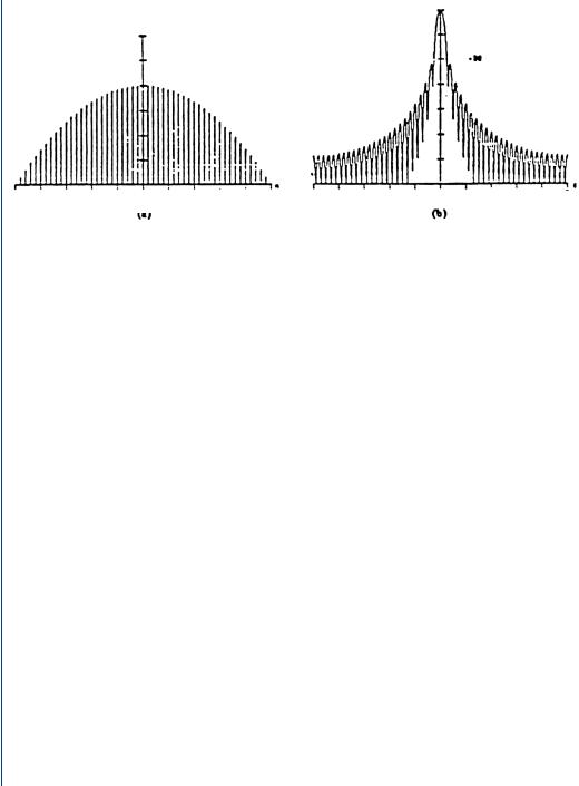
FIGURE 16.9: Fifty percent (50%) Tukey window. For alpha of 0.50, the trace (a) is the time domain weighted coefficients, whereas the trace (b) shows the main frequency lobe and the resulting side lobes. The first side lobe is −15 dBs from the peak of the frequency main lobe with a −18 dB per octave sidelobe fall-off rate

WINDOW FUNCTIONS AND SPECTRAL LEAKAGE 189

1 dB

1.2

–20

1.0

–40

0		T		–n bins
							n bins
					0
	(a)				(b)

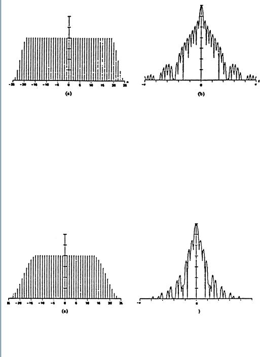
FIGURE 16.10: Seventy-five percent Tukey window. For alpha of 0.75, the trace (a) is the time domain weighted coefficients, whereas the trace (b) shows the main frequency lobe with the first side lobe at −19 dB and a −18 dB per octave side lobe fall-off rate

coefficients for alpha values of 1, 2, 3, and 4 are shown in Figs. 16.11(a), 16.12(a), 16.13(a), and 16.14(a), respectively. The resulting Log-magnitude of the Fourier transform for alpha values of 1, 2, 3, and 4 are shown in Figs. 16.11(b), 16.12(b), 16.13(b), and 16.14(b), respectively. Notice in the figures what effect increasing the value of alpha from 1 to 4 has on the first side-lobe value and the side-lobe roll-off rate. Note that for each increase of alpha by 1 the absolute magnitude of the side-lobe roll-off rate increases by 6 dB.

1.2
		–20
1.0
			–40

				–n bins
0	T				0
							n bins
(a)					(b)

FIGURE 16.11: Hanning window with alpha of 1. The trace (a) is the time domain weighted

coefficients, whereas the trace (b) shows the main frequency lobe with the first side-lobe at −23 dB

and a −12 dB per octave side-lobe fall-off rate

							1 dB
		1.2
						–20
		1.0
						–40

		–n bins
0	T			0	n bins
(a)				(b)

FIGURE 16.12: Hanning window with Alpha of 2. The trace (a) is the time domain weighted coefficients, whereas the trace (b) shows the main frequency lobe with the first side lobe at −32 dB and a −18 dB per octave side-lobe fall-off rate

1 dB

–20

1.2

1.0

–40

–60

0

T

n bins

–n bins

0

(a)

(b)

FIGURE 16.13: Hanning window with alpha of 3. The trace (a) is the time domain weighted coefficients, whereas the trace (b) shows the main frequency lobe with the first side lobe at −39 dB and a −24 dB per octave side-lobe fall-off rate

								1 dB
	1.2							–20
	1.0
								–40
								–60
0		T		–n bins		0
										n bins
(a)
						(b)

FIGURE 16.14: Hanning window with alpha of 4. The trace (a) is the time domain weighted coefficients, whereas the trace (b) shows the main frequency lobe with the first side lobe at −47 dB and a −30 dB per octave side-lobe fall-off rate