Brereton Chemometrics

APPENDICES	433

Figure A.9

Pseudo-inverse of a matrix

It is a very useful facility to be able to combine matrix operations. This means that more complex expressions can be performed. A common example is to calculate the pseudoinverse (Y .Y )−1.Y which, in Excel, is

=MMULT(MINVERSE(MMULT(TRANSPOSE(Y),Y)),TRANSPOSE(Y)).

Figure A.9 illustrates this, where Y is a 5 × 2 matrix, and its pseudoinverse a 2 × 5 matrix. Of course, each intermediate step of the calculation could be displayed separately if required. In addition, via macros (as described below) we can automate this to save keying long equations each time. However, for learning the basis of chemometrics, it is useful, in the first instance, to present the equation in full.

It is possible to add and subtract matrices using + and −, but remember to ensure that the two (or more) matrices have the same dimensions as has the destination. It is also possible to mix matrix and scalar operations, so that the syntax =2*MMULT(X,Y) is acceptable. Furthermore, it is possible to add (or subtract) matrices consisting of a constant number, for example =Y +2 would add 2 to each element of Y . Other conventions for mixing matrix and scalar variables and operations can be determined by practice, although in most cases the result is what we would logically expect.

There are a number of other matrix functions in Excel, for example to calculate determinant and trace of a matrix, to use these select the ‘Insert’ and ‘Function’ menus or use the Help system.

A.4.2.3 Arithmetic Functions of Scalars

There are numerous arithmetic functions that can be performed on single numbers. Useful examples are SQRT (square root), LOG (logarithm to the base 10), LN (natural logarithm), EXP (exponential) and ABS (absolute value), for example =SQRT(A1+2*B1). A few functions have no number to operate on, such as ROW() which is the row number of a cell, COLUMN() the column number of a cell and PI() the number π . Trigonometric functions operate on angles in radians, so be sure to convert if your original numbers are in degrees or cycles, for example =COS(PI()) gives a value of −1.

A.4.2.4 Arithmetic Functions of Ranges and Matrices

It is often useful to calculate the function of a range, for example =SUM(A1: C9) is the sum of the 27 numbers within the range. It is possible to use matrix notation so that =AVERAGE(X) is the average of all the numbers within the matrix X.

434	CHEMOMETRICS

Note that since the answer is a single number, these functions are not terminated bySHIFT CTL ENTER . Useful functions include SUM, AVERAGE, SUMSQ (sum of squares) and MEDIAN.

Some functions require more than one range. The CORREL function is useful for the chemometrician, and is used to compute the correlation coefficient between two arrays, syntax =CORREL(A,B), and is illustrated in Figure A.10. Another couple of useful functions involve linear regression. The functions =INTERCEPT(Y,X) and =SLOPE(Y,X) provide the parameters b0 and b1 in the equation y = b0 + b1x as illustrated in Figure A.11.

Standard deviations, variances and covariances are useful common functions. It is important to recognise that there are both population and sample functions, so that STDEV is the sample standard deviation and STDEVP the equivalent population standard deviation. Note that for standardising matrices it is a normal convention to use the population standard deviation. Similar comments apply to VAR and VARP.

Figure A.10

Correlation between two ranges

Figure A.11

Finding the slope and intercept when fitting a linear model to two ranges

APPENDICES	435

Note that, rather eccentrically, only the population covariance is available although the function is named COVAR (without the P ).

A.4.2.5 Statistical Functions

There are a surprisingly large number of common statistics available in Excel. Conventionally many such functions are presented in tabular format as in this book, for completeness, but most information can easily be obtained from Excel.

The inverse normal distribution is useful, and allows a determination of the number of standard deviations from the mean to give a defined probability; for example, =NORMINV(0.9,0,1) is the value within which 90 % (0.9) of the readings will fall if the mean is 0 and standard deviation 1, and equals 1.282, which can be verified using Table A.1. The function NORMDIST returns the probability of lying within a particular value; for example, =NORMDIST(1.5,0,1,TRUE) is the probability of a value which is less than 1.5, for a mean of 0 and standard deviation of 1, using the cumulative normal distribution (=TRUE), and equals 0.993 19 (see Table A.1). Similar functions TDIST, TINV, FDIST and FINV can be employed if required, eliminating the need for tables of the F statistic or t statistic, although most conventional texts and courses still employ these tables.

A.4.2.6 Logical Functions

There are several useful logical functions in Excel. IF is a common feature. Figure A.12 represents the function =IF(A1<B1,A1,B1) and places the lower of the values of columns A and B in column D. Note that this has been copied down the column and also that there are no $ signs in the arguments in this case. COUNTIF can be used to determine how many times an expression is valid within a region of a worksheet. This is useful, for example, to determine how many values of a matrix are above a threshold.

A.4.2.7 Nesting and Combining Functions and Equations

It is possible to nest and combine functions and equations. The expression =$C6 +

IF(A$7>1 ,10 ,IF(B$3 $C$2>5 ,15 ,0 ))ˆ2 −2 SUM SQ(X+Y ) is entirely legitimate, although it is important to ensure that each part of the expression results in an equivalent type of information (in this case the result of using the IF function is a number that is squared). Note that spreadsheets are not restricted to numerical information; they

Figure A.12

Use of I F in Excel

436	CHEMOMETRICS

may, for example, also contain names (characters) or logical variables or dates. In this section we have concentrated primarily on numerical functions, as these are the most useful for the chemometrician, but it is important to recognise that nonsensical results would be obtained, for example, if one tries to add a character to a numerical expression to a date.

A.4.3 Add-ins

A very important feature of Excel consists of Add-ins. In this section we will describe only those Add-ins that are part of the standard Excel package. It is possible to write one’s own Add-ins, or download a number of useful Add-ins from the Web. This book is associated with some Add-ins specifically for chemometrics as will be described in Section A.4.6.2.

If properly installed, there should be a ‘Data Analysis’ item in the ‘Tools’ menu. If this does not appear you should select the ‘Add-ins’ option and the tick the ‘Analysis Toolpak’. Normally this is sufficient, but sometimes the original Office disk is required. One difficulty is that some institutes use Excel over a network. The problem with this is that it is not always possible to install these facilities on an individual computer, and this must be performed by the Network administrator.

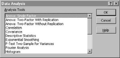
Once the menu item has been selected, the dialog box shown in Figure A.13 should appear. There are several useful facilities, but probably the most important for the purpose of chemometrics is the ‘Regression’ feature. The default notation in Excel differs from that in this book. A multiple linear model is formed between a single response y and any number of x variables. Figure A.14 illustrates the result of performing regression on two x variables to give the best fit model y ≈ b0 + b1x1 + b2x2. There are a number of statistics produced. Note that in the dialog box one selects ‘constant is zero’ if one does not want to have a b0 term; this is equivalent to forcing the intercept to be equal to 0. The answer, in the case illustrated, is y ≈ 0.0872 − 0.0971x1 + 0.2176x2; see cells H17 –H19 . Note that this answer could also have been performed using matrix multiplication with the pseudoinverse, after first adding a column of 1s to the X matrix, as described in Section A.1.2.5 and elsewhere. In addition, squared or interaction terms can easily be introduced to the x values, simply by producing additional columns and including these in the regression calculation.

Figure A.13

Data Analysis Add-in dialog box

APPENDICES	437

Figure A.14

Linear regression using the Excel Data Analysis Add-in

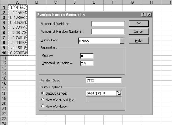
A second facility that is sometimes useful is the random number generator function. There are several possible distributions, but the most usual is the normal distribution. It is necessary to specify a mean and standard deviation. If one wants to be able to return to the distribution later, also specify a seed, which must be an integer number. Figure A.15 illustrates the generation of 10 random numbers coming from a distribution of mean 0 and standard deviation 2.5 placed in cells A1 –A10 (note that the standard deviation is of the parent population and will not be exactly the same for a sample). This facility is very helpful in simulations and can be employed to study the effect of noise on a dataset.

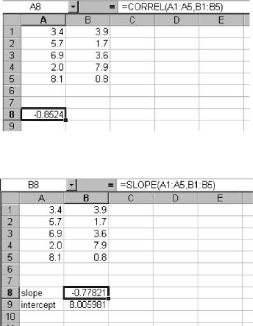
The ‘Correlation’ facility that allows one to determine the correlation coefficients between either rows or columns of a matrix is also useful in chemometrics, for example, as the first step in cluster analysis. Note that for individual objects it is better to use the CORREL function, but for a group of objects (or variables) the Data Analysis Add-in is easier.

A.4.4 Visual Basic for Applications

Excel comes with its own programming language, VBA (or Visual Basic for Applications). This can be used to produce ‘macros’, which are programs that can be run in Excel.

A.4.4.1 Running Macros

There are several ways of running macros. The simplest is via the ‘Tools’ menu item. Select ‘Macros’ menu item and then the ‘Macros’ option (both have the same name).

438	CHEMOMETRICS

Figure A.15

Generating random numbers in Excel

A dialog box should appear; see Figure A.16. This lists all macros available associated with all open XLS workbooks. Note that there may be macros associated with XLA files (see below) that are not presented in this dialog box. However, if you are developing macros yourself rather than using existing Add-ins, it is via this route that you will first be able to run home-made or modified programs, and readers are referred to more advanced texts if they wish to produce more sophisticated packages. This text is restricted to guidance in first steps, which should be sufficient for all the data analysis in this book. To run a macro from the menu, select the option and then either double click it, or select the right-hand-side ‘Run’ option.

It is possible to display the code of a macro, either by selecting the right-hand-side edit option in the dialog box above, or else by selecting the ‘Visual Basic Editor’ option of the ‘Macros’ menu item of the ‘Tools’ menu. A screen similar to that in Figure A.17 will appear. There are various ways of arranging the windows in the VB Editor screen, and the first time you use this feature the windows may not be organised in exactly as presented in the figure; if no code is displayed, you can find this using the ‘Project Explorer’ window. To run a procedure, either select the ‘Run’ menu, or press the symbol. For experienced programmers, there are a number of other ways of running programs that allow debugging.

APPENDICES	439

Figure A.16

Macros dialog box

Figure A.17

VBA editor

Macros can be run using control keys, for example, ‘CTL’ ‘f’ could be the command for a macro called ‘loadings’. To do this for a new macro, select ‘Options’ in the ‘Macro’ dialog box and you will be presented with a screen as depicted in Figure A.18. After this, it is only necessary to press the CTL and f keys simultaneously to run this

440	CHEMOMETRICS

Figure A.18

Associating a Control key with a macro

macro. However, the disadvantage is that standard Excel functions are overwritten, and this facility is a left-over from previous Excel versions.

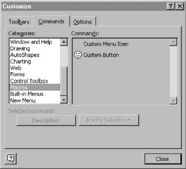
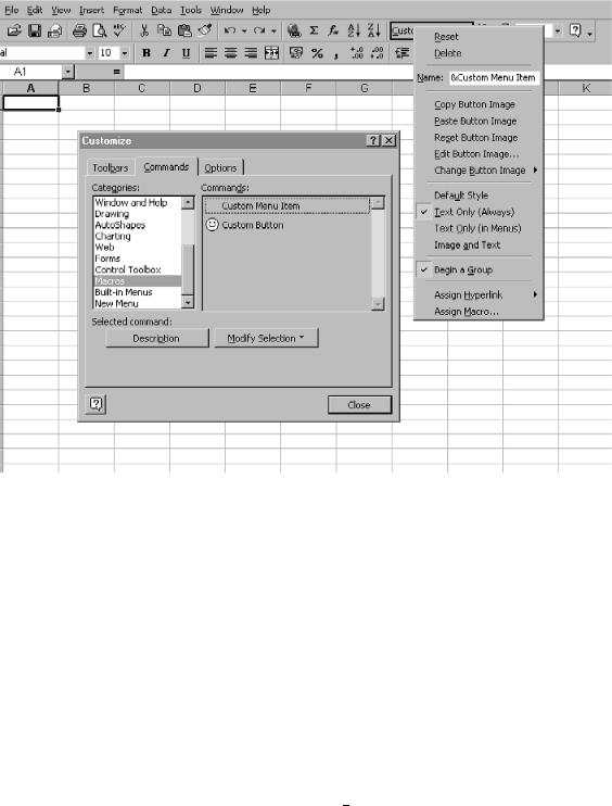
A better approach is to run the macro as a menu item or button. There are a number of ways of doing this, the simplest being via the ‘Customize’ dialog box. In the ‘View’ menu, select ‘Toolbars’ and then ‘Customize’. Once this dialog box is obtained, select the ‘Commands’ and ‘Macros’ options as shown in Figure A.19. Select either ‘Custom Button’ or ‘Custom Menu Item’ and then drag to where you wish it. Right clicking whilst the ‘Customize’ menu is open allows the properties of the button or menu item to be changed; see Figure A.20. The most useful are the facilities to ‘Assign Macro’ or to change the name (for a menu item). Some practice is necessary to enable the user to place macros within menus or as buttons or both, and the best way to learn is to experiment with the various options.

A.4.4.2 Creating and Editing Macros

There are a number of ways of creating macros. The most straightforward is via the Visual Basic Editor, which can be accessed via the ‘Macro’ option of the ‘Tools’ menu. Depending on your set-up and the history of the spreadsheet, you may then enter a blank screen. If this is so, insert a ‘Module’. This contains a series of user defined procedures (organised into Subroutines and Functions) that can be run from Excel.

APPENDICES	441

Figure A.19

Associating a macro with a menu item or a button

It is possible to have several modules, which helps organisation and housekeeping during programming, but the newcomer will probably wish to keep this aspect simple at first. Using the ‘View’ menu and ‘Project Explorer’, it is possible to obtain a window with all the open modules and workbooks, allowing reorganisation and renaming of modules; this is illustrated in Figure A.21.

Creating a new macro that is called directly from Excel is simple. In the code window, on a new line, type Sub followed by the macro name and terminated by a carriage return. VBA will automatically create a new macro as illustrated in Figure A.22 for a subroutine Calc. All subroutines without arguments may be called by Excel. Subroutines with arguments or functions are not able to be directly called by Excel. However, most programs of any sophistication are structured, so it is possible to create several procedures with arguments, and use a small routine from Excel to call these. To develop the program, simply type statements in between the Sub and End Sub statements.

There are a number of ways of modifying existing procedures. The most straightforward is in the Visual Basic Editor as discussed above, but it is also possible to do this using the ‘Macro’ option of the ‘Tools’ menu. Instead of running a macro, choose to ‘Edit’ the code. There are numerous tricks for debugging macros, which we will not cover in this book. In addition, the code can be hidden or compiled. This is useful when distributing software, to prevents users copying or modifying code. However, it is best to start simply and it is very easy to get going and then, once one has developed a level of expertise, to investigate more sophisticated ways of packaging the software.

442	CHEMOMETRICS

Figure A.20

Changing the properties of a menu item

Another way of creating macros is by the ‘Record New Macro’ facility, which can be entered via the ‘Macro’ option of the ‘Tools’ menu. This allows the user to produce a procedure which exactly corresponds to a series of operations in Excel. Every facility in Excel, whether changing the colour of a cell, multiplying matrices, changing the shape of a symbol in a graph or performing regression, has an equivalent statement in VBA. Hence this facility is very useful. However, often the code is rather cumbersome and the mechanisms for performing the operations are not very flexible. For example, although all the matrix operations in Excel, such as MMULT, can, indeed, be translated into VBA, the corresponding commands are tricky. The following is the result of

•multiplying the transpose of cells B34 to B65 (a vector of length 32) by

•cells C34 to C65

•and placing the result in cell E34 .

Selection.FormulaArray =

"=MMULT(TRANSPOSE(RC[-3]:R[31]C[-3]),RC[-2]:R[31]C[-2])"