64 DETERMINATION OF COMPLEX REACTION MECHANISMS

simultaneously. They may affect the stoichiometry, particularly at branching points, as we observed for the two molecules of DHAP produced from one molecule of F1,6BP.

Acknowledgment This chapter is based on the article “Experimental test of a method for determining causal connectivities of species in reactions” by Antonio Sanchez Torralba, Kristine Yu, Peidong Shen, Peter Oefner, and John Ross [1], with minor changes in wording.

Reference

[1]Sanchez Torralba, A.; Yu, K.; Shen, P.; Oefner, P. J.; Ross, J. Experimental test of a method for determining causal connectivities of species in reactions. Proc. Natl. Acad. Sci. USA 2003, 100, 1494–1498.

7

Correlation Metric Construction

Theory of Statistical Construction of

Reaction Mechanisms

In chapter 5, we studied the responses of chemical species in a reaction system to pulse perturbations and showed the deduction of direct, causal connectivities by chemical reactions—the reaction pathway—and the reaction mechanism from such measurements. The causal connectivites give the information on how the chemical species are connected by chemical reactions. In this chapter we turn to another source of information about chemical species in a reaction system, that of correlations among the species.

Correlations of concentrations are measures of the statistical dependence of the concentration of one species on that of one or more of the other species in the system. Such correlations can be determined from measurements of time series of concentrations collected around a stationary state (nonequilibrium or equilibrium). We shall show that from concentration correlations it is possible to construct a skeletal diagram of the reaction system that gives a graphical measure of strong control and regulatory structure in reaction networks, gives some information on connectivity, leads to information on the reaction pathway and mechanism, and may simplify the analysis of such networks by identifying possible, nearly separable subsystems [1].

We begin with the demonstration and explanation of this approach by analyzing some abstract reaction models. In chapter 8 we show the utility of this “correlation metric construction” (CMC) with application to time-series measurements on a part of glycolysis, and in chapter 13 on an extensive genome study.

Consider a chemical system as shown in fig. 7.1. Mechanisms of this type are common in biochemical networks. For example, the subnetwork of fig. 7.1 containing S3 to S5 is based on a simple model of fructose interconversion in glycolysis [2] (see fig. 1.2) and the subnetwork composed of S6 to S7 is similar to the phosphorylation/dephosphorylation cycles found in cyclic cascades [3,4]. As an aside, this mechanism performs the function

65

66 DETERMINATION OF COMPLEX REACTION MECHANISMS

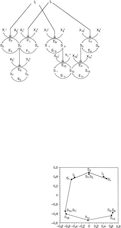
Fig. 7.1 Chemical reaction mechanism representing a biochemical NAND gate. At steady state, the concentration of species S6 is low if and only if the concentrations of both species I1 and I2 are high. All species with asterisks are held constant by buffering. Thus, the system is formally open although there are two conservation constraints. The first constraint conserves the total concentration of S3 + S4 + S5, and the second conserves S6 + S7. All enzyme-catalyzed reactions in this model are governed by simple Michaelis–Menten kinetics. Lines ending in over an enzymatic reaction step indicate that the corresponding enzyme is inhibited (noncompetitively) by the relevant chemical species. We have set the dissociation constants, KD,i , of each of the enzymes E1–E6, from their respective substrates equal to 5 concentration units. The inhibition constants, K11 and K12, for the noncompetitive inhibition of E1 and E2 by I1 and I2, respectively, are both equal to 1 unit. The Vmax for both E1 and E2 is set to 5 units, and that for E3 and E4 is 1 unit/s. The Vmax ’s for E5 and E6 are 10 and 1 units/s, respectively. (From [1].)

of a biochemical NAND gate, another example of a chemical computational function (see chapter 4). The goal of CMC is to determine both the regulatory structure and the connectivity of the species in the elementary reaction steps of this mechanism, solely from measurements of the responses of the concentrations of S3 to S7 to externally imposed variations in the input concentrations, I1 and I2. The choice of input species and response species is arbitrary but may be influenced by some prior knowledge of the system. In the system in fig. 7.1 we have a total of 7 species. We assume initially that it is possible to identify and measure all the chemical species that make up the chemical network. This is a strong assumption, but with continuing improvements in instrumentation it is increasingly satisfied. Further, we assume that we may impose concentration variations independently on a subset of chemical species in the network at each time.

If the system is initially in a stationary state, then the imposition of concentration variations of I1 and I2 will remove the system from that stationary state and, after a given variation, the system returns to the stationary state with a given relaxation time. The differences in time between adjacent concentration measurements are assumed to be on the order of, or longer than, the slowest relaxation time in the network. If the differences in time are much shorter than the relaxation time, the system cannot respond; the system will act as a low-pass filter and degrade the input signal. On the other hand, if the intervals in time are too long, then the system returns to its stationary state. Some filtering—degrading of the signal—must occur to obtain information on the correlations from the time series.

The imposed concentration variations can be chosen; for example, they can be periodic or random. We shall choose them to be random. The procedure of CMC requires

CORRELATION METRIC CONSTRUCTION

67

several steps which we now detail.

1.The set of measurements of the concentrations of the species in Si is obtained as a function of the externally controlled concentrations of the species I1 and I2 at each of the selected time points. Figure 7.2 is a plot of the time series for each of the species in this system. One time point is taken every 10 s for 3,600 s. The effects of using a much smaller set of observations are discussed later. The first two plots are the time series for the two externally controlled inputs. The concentrations of I1 and I2 at each time point are chosen from a truncated Gaussian (normal) distribution centered at 30 concentration units with a standard deviation of 30 units. The distribution is truncated at zero concentration. The choice of Gaussian noise guarantees that in the long time limit the entire state-space of the two inputs is sampled and that there are no autocorrelations or cross-correlations between the input species. Thus all concentration correlations arise from the reaction mechanism. The bottom five times series are the responses of the species S3 to S7 to the concentration variations of the inputs.

It is interesting to note in fig. 7.2 that this chemical system, as in many if not most other reactions, acts a frequency filter; much of the higher frequency noise in the two inputs I1 and I2 is filtered out in the responses, the more so the further the response species is separated from the input species by reactions. For more discussion on this subject see [5].

2.From the measured (in this case calculated) time series of the concentrations in

fig. 7.2 we form correlation functions. Denote by xi (t) the concentration of species Ii at time t, and by xi the average of that concentration over the entire time of the measurements; then the time-lagged correlation function of two species i and j, Sij (τ ), is defined by

Sij (τ ) = (xi (t) −		i )(xj (t + τ ) −		j )	(7.1)
	x		x

for a given time lag τ , which may be positive, negative, or zero. If the random variations of I1 and I2 affect the concentration of species i independently from that of species j, then the correlation function Sij (τ ) is zero for any value of τ . We have so far introduced only pair correlation functions for two species at a time. This measure of association is, in many ways, a precursor of later methods that utilize higher moments of the joint probability distribution among the system variables. We discuss one of these extensions at length in chapter 9 and another related approach in chapter 13 (see section 13.6, “Bayesian Networks”).

It is convenient to discuss normalized correlation functions rij , defined by the equation

rij (τ ) =	Sij (τ )	(7.2)
	Sii (τ ) Sjj (τ )

The indices i and j range over all species in the system.The correlation functions depend in a complicated way on the elementary reactions and their rate coefficients.

There are two conservation constraints in this system: first, the sum of the concentrations of S6 and S7 is constant; second, the sum of the concentrations of S3, S4, and S5 is constant. Hence of the 5 response concentrations, only 3 are independent; the matrix R made up of the correlations rij is four-dimensional, three concentration dimensions and the time lag τ .

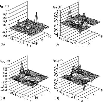
Figure 7.3 is a set of plots of some three-dimensional cross-sections from the four-dimensional R(τ ) surface calculated from the data in fig. 7.2. Each crosssection represents the correlations, at all calculated time lags (here every ±10 s up to

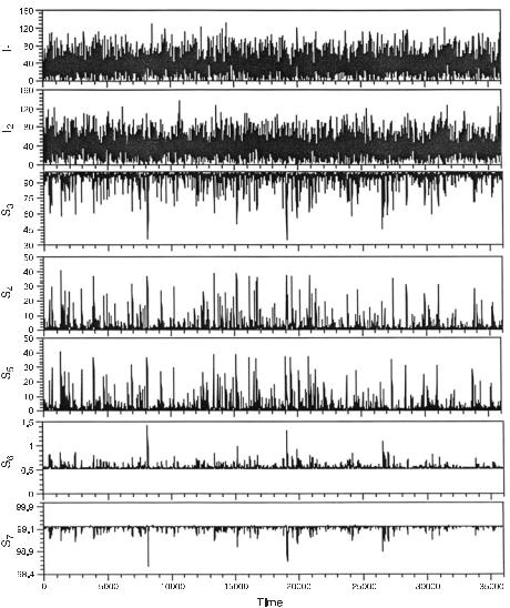
Fig. 7.2 Plot of the calculated concentration time series for all the species composing the mechanism in fig. 7.1. Only the first two time courses (those for I1 and I2) are set by the experimenter. The concentrations of I1 and I2 are chosen independently from a Gaussian distribution with a mean and standard deviation of 30.0 concentration units. Since the lower limit of concentration is zero, the actual distribution of input concentrations has a tail toward high concentrations. See step 1 in the text for a full explanation. (From [1].)

CORRELATION METRIC CONSTRUCTION

69

Fig. 7.3 Plots of cross-sections through the four-dimensional time-lag correlation surface calculated from eqs. (7.1) and (7.2). The cross-sections are A = r1, j (t), B = rS3 , j (t), C = rS4 , j (t), and D = rS6 , j (t). See step 2 in the text for explanation. (From [1].)

a time lag of ±190 s), of the times series corresponding to a given species with those of each of the other species, and itself. If the system were truly at steady state at each time point, then the correlation surface for combinational networks (those in which there are no feedback loops) would be flat except on the τ = 0 plane. Figure 7.3 shows only four cross-sections corresponding to the choice of three independent species and one of the inputs. Examination of the cross-sections of R(τ ) (fig. 7.3D) shows that, as expected, the concentration of S6 perfectly anticorrelates with that of S7 (by conservation) and negatively correlates with that of S3.

Figure 7.4 shows two projections of the cross-sections in fig. 7.3B. Figure 7.4A is a projection on the species correlation plane. This projection shows the relative correlations of each of the species with S3. Figure 7.4B is a projection on the time-lag correlation plane. Here, a rough sequence of events in time becomes clear when it is noted that if one species correlates with a second species at a positive lag, then the variation of the first species occurs (on average) before that of the second. The correlation of a species with itself at nonzero lag is expected due to relaxation to the steady state and should be symmetric around zero lag. The sequence of events with respect to S3 is therefore as follows: I1 and I2 are changed externally, followed by the simultaneous changes in S3 to S5, after which S6 and S7 change. In this case, this time line is a sequence of causal connectivity. However, in branched networks or networks with feedback, causal connectivity may not always be determined in

70 DETERMINATION OF COMPLEX REACTION MECHANISMS

Fig. 7.4 Projections of fig. 7.3B down the species (A) and time-lag (B) axes. Figure 7.4A emphasizes the correlation of S3 with all the other species. It correlates most highly with S6 and S7, next with S4 and S5, and finally with I1 and I2. Figure 7.4B (truncated to emphasize the region between t = ±10 units) shows the large amount of time information that is largely ignored by the simple analysis presented here. If a species correlates at a positive lag with respect to S3, then that species leads S3 in time; a negative lag implies that the correlating species follows S3. Since fig. 7.4B shows that the correlation with the inputs tails toward positive lags, action on the inputs precedes action at S3. Action at S4 and S5 occurs simultaneously with S3, and S6 and S7 follow action at S3 (as indicated by their left tails). In this particular network this sequence of lags relates directly to the causal sequence. The inputs affect the concentration of S3–S5, which then affects the concentration of S6 and S7. The amount of this information available for a given experiment is dependent on the magnitude of the rate coefficients with respect to the time between measurements. (From [1].)

this way. Further, if the time between measurements had been 70 s rather than 10 s, the network would have been at steady state and no time delays would be observed.

Causality, in this case the assignment of which reactants lead to which products, cannot be determined simply by the strength of a statistical relation. Three criteria must be met for causality to be established: there must be (1) a temporal ordering of the variables; (2) concomitant variation; and (3) control over other factors that might affect the observed relationships among the variables. In CMC we do not always meet the first criterion, and the third criterion can only be fulfilled by data outside the present analysis, for example, knowledge of the basic chemistry. This point is especially relevant to the connection algorithm discussed in step 3.

The correlation matrix is symmetrical with 1’s on the diagonal. If two or more covariates are perfectly correlated, this implies that there will be columns and rows of the correlation matrix that are exactly the same. Thus the correlation matrix will not be of full rank. In noiseless experiments, perfect correlation can arise for a number of reasons. The two most common would be the existence of a conservation condition among two or more species and the establishment of quasi-equilibria. In the case of conservation, the decrease in one concentration is necessarily followed by the increase in others. For two species in a conservation relationship this results in perfect anticorrelation between the variates. For quasior actual equilibria the

CORRELATION METRIC CONSTRUCTION

71

input signal has effectively propagated instantaneously throughout the system; thus, since the final concentration of each species in the “equilibrium relationship” will be a function only of the kinetic parameters and the current value of the inputs (but not time), their dynamics will be perfectly correlated (unless there is no variation in one of the concentrations). In our examples there are a number of such conditions.

The nullity (the number of zero eigenvalues) and null-space (the space spanned by the corresponding eigenvectors) of the correlation matrix determine the number of conservation constraints and rapidly established quasi-equilibria in the network and the species involved, respectively (since species involved in such relations are completely dependent on one another). For example, the eigenval-

ues of the (zero lag) correlation matrix derived from the time series in fig. 7.3 are A = (3.89, 1.3, 0.97, 0.67, 0.17, 1.7 × 10−7, 7.0 × 10−9). Thus, since the last

two eigenvalues are so small compared to the first five, the nullity of the matrix is 2, as expected from the two conservation conditions. The correlation matrix can be cleaned up somewhat by zeroing all correlations that are not significant by the standard t-statistic-based significant tests [6].

3.We suggest a connection algorithm which generates an approximate dependency list among the different species. Ideally, we would like the dependency list to reflect directly the reactions among the species. However, dependency as obtained from the correlation studies is not necessarily related to causal connectivity, but rather to a high degree of association among sets of variables . There are a number of common analyses, such as multiple regression, canonical correlation [7], linear structural relation (LISREL or SEPATH) [8,9], and Box–Jenkins time-series analysis [10], which attempt to determine the dependencies of a set of observable dependent variables on known independent variables. All of these techniques are essentially regression analyses in which an estimate of the mean of one set of variables is made based on knowledge of another set of variables.

In each of the cases above, a general model structure is asserted. An example is

a simple nonlinear regression (as discussed in chapter 1) in which the observation of one variation at time t is dependent on other variables at time time t − τ . A simple regression model might look like eq. (1.1), where the regression methods solve for the β’s which are conceptually (and sometimes actually) related to our correlation measures of association. This example is relatively unstructured and methods like LISREL allow the assertion of more causal hypotheses into the regression. One goal of CMC is to construct an approximate model of the interactions among species, without explicit specification of a model (chemical mechanism). Correlation-based analysis measures a symmetric degree of association between two variables. Thus, correlations yield a convenient metric of distance between two species. Since the balance of our method (steps 4–7) relies on such a metric, we develop a simple correlation-based agglomerative dependency algorithm with the following iterated steps that are very similar to the procedures one would use to hierarchically cluster the data:

(a)Place each species in its own group.

(b)Find the two groups, i and j, each containing a disjoint subset of species for which the magnitude of correlation (at any lag) between a species in i and one in j is the maximum over all pairs of groups. That is, find the maximum correlation between two species not in the same group.

(c)Merge these two groups into one group and list the connection, found in step (b), between the two species (one from each original group) with the maximum correlation. If two or more species from one group correlate with species in the other with (nearly) the same maximum magnitude, then list connections

72 DETERMINATION OF COMPLEX REACTION MECHANISMS

between these as well. All listed connections are designated as “significant” connections, since we did not reject the correlation by the t-statistic mentioned above.

(d)Go back to (b), now with one fewer group, and repeat the steps until there is only a single group left. This procedure creates a singly linked system graph in which every species is connected to at least one other species.

Application of the connection algorithm to the full correlation surface of the NAND mechanism yields the values of the significant connections listed in table 7.1. The algorithm neglects the direct effect of each input species on the concentration of S3 since we are using only a single-link dependency; the magnitude of the correlation between the inputs and S3 is weak since S3 is maximally affected only when the inputs are both low or both high at the same time (a relatively rare event). It may be possible to eliminate such statistical misses and redundancies in the connection list by including chemical knowledge, incorporating the available correlation time-lag information, and application of the transinformation criterion of probabilistic reconstruction analysis, a variant of which we use in EMC and ERT, discussed in chapter 9, which uses conditional probabilities derived from the full (calculated) joint probability density function generated from the time series. Lastly, the difference in correlations of S4 and S5 to S3 is merely a result of the sampling statistics. There is also a standard t-statistic to test for the significance of the difference for two correlations drawn from the same experimental data.

The connections among species, since they are based on correlations, represent a noncausal structural model of the system. Correlations may be decomposed into four parts: (1) direct effects, that is, causal connectivity, in which one variable is a direct antecedent to a second (e.g., one species is directly converted to another by a chemical reaction); (2) indirect effects, where one variable influences another by way of a third (e.g., one species affects the production of a second which is then converted directly to a third); (3) spurious effects, which occur when two variables have a common antecedent (e.g., when one species is converted into two other species by separate reactions); and (4) unanalyzed effects, which arise from correlations between the externally controlled variables [11]. In order to construct a mechanism (a causal model), only the first contribution to the correlation between two variables should be considered. We do not here separate the measured correlation into these explicit components. In the absence of special knowledge of the chemical mechanism, methods for doing so, such as path analysis and LISREL [8,9], require extensive and complex calculation as well as a number of restrictive assumptions. Our simple definition of connection, though possibly not as informative as a full analysis of causal connectivity, yields a good first guess for a relational structure among the species (ideally defined by the first component of correlation above).

Table 7.1 Listing of the “significant” connections calculated among the chemical species composing the reaction mechanism in fig. 7.1

	S4	S5	S6	S7
I1	−0.31	−0.32
I2	−0.72		−0.90
S3		−0.71		0.90
S6				−1.00

CORRELATION METRIC CONSTRUCTION

73

A partial description of the functions of the network may be read from the signs of the connections in table 7.1. For example, since I1 and I2 are negatively correlated with S4 and S5, both of which are negatively correlated with S3, we may hypothesize that S3 is high only when I1 or I2 or both are high, and S3 is low otherwise. So the subsystem of fig. 7.1 composed of S3–S5, and with the output defined as S3, may be functionally analogous to a logical OR (or an AND) gate between I1 and I2. In this particular case, the function is an AND gate. If only I1 is high, then material partitions between S3 and S5, and if only I2 is high, then material partitions between S3 and S4. If I1 and I2 are both high, then all materials funnel toward S3. If the kinetics are set up correctly (reaction from S3 → S4, S5 fast without I1,2 and very slow with I1,2), then this arrangement accumulates S3 only when I1 and I2 are both high.

4.The time-lagged correlation matrix, R(τ ), is converted into a Euclidean distance matrix with the canonical transform [7]:

dij

=

cii − 2cij + cjj

1/2

= 21/2

1.0 − cij

1/2

(7.3)

ij

=

|

ij (τ )

|

τ

c

max

r

(7.4)

where the second equality in eq. (7.3) follows from the properties of the correlation matrix. The formula in eq. (7.4) defines cij to be the absolute value of the maximum correlation between the time series for species i and that of species j, regardless of the value of τ . The neglect of the value of τ at the maximum correlation between two time series represents a loss of useful information. In kinetic systems in which the correlation is peaked at some nonzero lag, the implication is that that the system is large enough, in the sense of sufficient species, for there to be a delay time between the site of signal generation (the inputs) and the reception. This information may be incorporated into the distance metric in order to represent better the distances among the species, In addition, the sign of the lag may be used to estimate a sequence of events.

We define D = (dij ) to be the distance matrix. Since D is Euclidean, its elements automatically satisfy the three standard tests for a metric space: identity, symmetry, and the triangle inequality. In the case of perfect correlation between two variables, the triangle inequality is violated, a situation that may be remedied (without dire consequences) by adding a small value, ε = 1 × 10−10, to the distance between them. The particular metric defined by eq. (7.3) is a measure of independence between two variables. If the correlation between two variables is small, then the distance between them is large.

5.The classical multidimensional scaling (MDS) method [7,12] is applied to the distance matrix calculated in step 4 in order to find both the dimensionality, , of the system and a consistent configuration of points representing each of the species. Before explaining the mathematics of that process, let us give a pictorial representation. Think of each of the significant connections in table 7.1 as represented by a stick: the length of the stick is determined by the absolute magnitude of the correlation listed in the table and the stick carries a label of one species at one end and that of another species at the other end. For example, for the correlation of species S3 and S5 the stick has a length of 0.71 and is marked at one end with S3 and at the other end with S5. Now take the 7 sticks corresponding to the 7 entries in the table, pick out all those with I1 on one end, and place those ends at one point. Next, do the same for all ends marked I2, and so on. You will need a multidimensional space to accomplish this, but you will have constructed a multidimensional object. Shine a beam of light on the object and observe the projection of the object on a screen.

74 DETERMINATION OF COMPLEX REACTION MECHANISMS

Rotate the object until the information that you have about the object on the screen is a maximum. For the case of the object built from the entries of correlations in table 7.1 the best projections are given in fig. 7.5, which displays well the reaction pathway of the mechanism in fig. 7.1.

To accomplish the task just described mathematically, we use a standard approach by defining a centered inner product matrix B by the equations

B = −(1/2)H(dij )H	(7.5)
H = I − (1/M)II	(7.6)

where H is the centering matrix [7], I is the M × M identity matrix, and II is the M × M unit matrix. The operation of the symmetric, idempotent matrix H on the vector x has the effect of subtracting off the mean of the entries of x from each of its elements, that is, Hx = x − x I, where x = n−1 xi . The number of significant eigenvalues of B (defined in table 7.2) is the dimensionality, , of the system, and the vectors constructed from the first coordinates of the M eigenvectors comprise the principal coordinates of points representing the chemical species in the correlation diagram. (Formally, each point represents the particular time series generated for a given chemical species.) The eigenvectors are normalized such that zi · zi = λi . The distance between each pair of points is inversely related to the correlation between the corresponding species. If the M series are independent, then all the dij are equal to 21/2 and points representing each species must fall on the vertices of a regular M − 1-dimensional hypertetrahedron. At the other extreme, when all species perfectly correlate (or anticorrelate), then the dij are all equal to 0 and there is a single degenerate point in the system. By construction, however, the inputs are completely uncorrelated, so the minimum dimension derived from a CMC is |I | − 1. Most often, we are interested in the first two principal coordinates of the MDS solution since the configurations may then be plotted on a plane and are thus easy to visualize.

The numerical results from the MDS analysis of the distance matrix derived from eqs. (7.3) and (7.4) are shown in table 7.2. The columns of table 7.2A are the eigenvectors of B, and the rows are the coordinates of each point (time series). Each eigenvector, zk , corresponds to the projection of the kth coordinate of each of the points on an orthogonal basis vector. Each of the eigenvalues (table 7.2B) is an indicator of the degree to which the vectors from the origin of the configuration to each point are projected along the corresponding basis vector. In this example, over 99% (for a2,3) of the distance matrix is “explained” by the first three eigenvalues. Thus, we find the dimensionality ≈ 3, which represents a reduction of three dimensions from the theoretical maximum of six. Two of these dimensions are lost due to the two conservation constraints. The third dimension is lost due to constraints imposed by the degree of interaction among the subsystems (the conservation conditions lead to a degeneracy in the correlation matrix). The twodimensional projection of the coordinates of the points listed in table 7.2A is shown in fig. 7.5A. Each pair of points with a nonzero entry in table 7.1 is connected by a line. This represents the correlation metric diagram which depends on the reaction mechanism and rate coefficients (as well as the properties of the perturbations, such as the frequency spectra, average values, and standard deviations). This diagram reproduces many features of the standard mechanistic diagram (fig. 7.1) but

CORRELATION METRIC CONSTRUCTION

75

Table 7.2 Eigenvectors and eigenvalues of the matrix B (eq. 7.5) determined by the classical MDS analysis of a distance matrix calculated from the correlation surface in fig. 7.3 (see steps 4 and 5 in the text)

(A) Eigenvectors, zk :

Point/zk		1	2	3	4	5	6	7
1	(I1)	6.68e−01	−5.84e−01 4.05e−01		5.51e−02	1.77e−02 −8.20e−09 −3.52e−10
2	(I2)	7.00e−01	5.26e−01 −4.30e−01		4.93e−02	1.42e−02 −8.20e−09 −3.52e−10
3	(S7)	−4.20e−01	7.29e−03 −8.16e−03		2.05e−01	1.90e−03	−6.82e−09 −7.67e−09
4	(S6)	−4.20e−01	7.29e−03	−8.16e−03	2.05e−01	1.90e−03	−9.58e−09	6.97e−09
5	(S4)	−1.44e−01	−5.51e−01 −4.02e−01 −1.60e−01 −7.55e−02 −8.20e−09 −3.52e−10
6	(S5)	−7.15e−02	5.60e−01	4.30e−01	−1.38e−01	−7.65e−02 −8.20e−09		−3.52e−10
7	(S3)	−3.14e−01	3.49e−02	1.27e−02	−2.16e−01	1.16e−01	−8.20e−09	−3.52e−10

(B) Eigenvalues, λk :

k	λk	a1,k	a2,k
1	1.413496e+00	3.978311e−01	4.937104e−01
2	1.237497e+00	7.461268e−01	8.721279e−01
3	6.958617e−01	9.419783e−01	9.917824e−01
4	1.805556e−01	9.927960e−01	9.998381e−01
5	2.559576e−02	1.000000e+00	1.000000e+00
6	4.747935e−16	1.000000e+00	1.000000e+00
7	1.080736e−16	1.000000e+00	1.000000e+00

The coefficients a1,k and a2,k are agreement measures of the degree to which the distance matrix is “explained” by the k-dimensional MDS solution. The measures are calculated from

		k					k
			λi				λi2
	=					=
a1,k		i=1		and	a2k		i=1
		n	|λi |				n
							λi2
		i=1					i=1

where the eigenvalues are sorted in decreasing order. Thus, according to a2,k , 49.4% of the distance matrix is explained by one dimension (a2.1 = 0.494) and 100% of the matrix is explained by a configuration in five dimensions (a2.5 = 1.0). Columns 1 and 2 of the eigenvector matrix define the x and y positions of points in fig. 7.4A, respectively.

differs in that it has additional information, such as the extent of coupling (tightly or loosely) among subsystems in the network.

6.Figure 7.5A is a projection of the high-dimensional MDS object onto two dimensions. The distances between the points in the 2D representation are therefore less than or equal to actual measured distances. A more representative 2D diagram may often be obtained with an optimization-based MDS method that allows the distances between the optimized points to be greater than, equal to, and less than the actual distances (see [11]). The diagram derived with this algorithm from our example is shown in fig. 7.5B, which is more representative of the actual distance

76 DETERMINATION OF COMPLEX REACTION MECHANISMS

Fig. 7.5 Classical and optimized MDS solutions calculated from the canonically transformed correlation surface from fig. 7.3. (A) The two-dimensional projection of the three-dimensional (a2,3 = 99.2%) (or four-dimensional; a2,4 = 99.98%) object found by the matrix method described by step 5 in the text. The coordinates for the points in A are the same as the first two columns of the matrix of eigenvectors in table 7.2A. The second diagram (B) is derived from the MDS optimization method discussed in step 6. The lines between points in both diagrams are obtained from the results of step 3 (table 7.1). Thus, B is more representative of the measured distance matrix. Both diagrams correspond to rotated and slightly distorted approximations to the reaction mechanism in fig.7.1. (From [1].)

matrix (see the caption of fig. 7.5). Note that all rotations, reflections, and translations of the MDS diagrams are equally valid MDS solutions. Both diagrams, parts A and B of fig. 7.5, are rotated and slightly distorted versions of the diagram of the reaction mechanism shown in fig. 7.1. Thus, from the state measurements (calculations) of the time series, we derive a construction related to the reaction mechanism for the system, but with the added information on the relative coupling strengths among species.

7.Finally, a cluster analysis is performed on the distance matrix. This method is used to summarize the grouping of chemical subsystems within the reaction mechanism and to give a hierarchy of interactions among the subsystems. There are many techniques of cluster analysis [7,12,13], but for simplicity we employ a nonparametric hierarchical clustering technique called the weighted pair group method using arithmetic averages [14]. The algorithm operates on D in three iterated steps:

(a)Search the M × M distance matrix for the minimum distance between pairs of clusters and let this distance be dij . In the initial step, there are M clusters (u1, u2, . . . , uM ) each containing a single point (species).

(b)Define a new cluster, uk , containing the two objects (i and j) with the minimum distance between them. Define the branching depth of this cluster as hij =

dij /2. Finally, define the distance between the new cluster, k, and all other clusters, l = i or j , by the equation dkl = (dil + dik )/2.

CORRELATION METRIC CONSTRUCTION

77

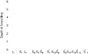
Fig. 7.6 Hierarchically clustered dendrogram calculated from the CMC analysis of the mechanism in fig. 7.1. The dendrogram is produced as described in step 7 in the text. The hierarchy is a good representation of the flow of control from the inputs down to S6 and S7. (From [1].)

(c)Delete clusters i and j from the distance matrix and add the newly computed cluster distances to the matrix. If M is not equal to 1, then decrease M by one and return to step 1, otherwise the algorithm is done.

This procedure generates a dendrogram. Such dendrograms have also been used to visualize and aid interpretation of the results of microarray experiments [15]. The dendrogram derived from a cluster analysis of the distance matrix calculated in step 4 is shown in fig. 7.6. The tree may be interpreted as follows. Since the branching depths of species I1 and I2 are nearly the same, but they do not belong to the same cluster, we may consider the two as separate subsystems which couple with similar strengths to the rest of the network (the species below the inputs in the diagram). A similar assumption may be made about species S4 and S5. The diagram is then simple to analyze. Since we control species I1 and I2, these in turn most strongly influence the changes in concentrations of both S4 and S5. These two species then combine to control the concentrations in the subnetwork (S3, S6, S7). This three-member subnetwork may be further divided into S3 and (S6, S7). From the correlation metric diagram and the eigenanalysis of the correlation matrix we know that S4 and S5 are the determinants of S3 (since the connections are significant and the three species are involved in a conservation relation), which subsequently controls the concentrations of S6 and S7. These last two species also satisfy a conservation constraint. Thus, a hierarchical diagram of control is derived.

We next discusss some more examples in order to clarify the usage and interpretations of CMC analyses. Figure 7.7 shows a chemical system composed of two subsystems, one like that of fig. 7.1 (subsystem 1) and another realizing a NOT I1 and NOT I2 function (subsystem 2). The kinetics of subsystem 1 are chosen to be faster than the analogous system in fig. 7.1. Subsystem 2 is composed of substrate cycles similar to those in subsystem 1, but the kinetics of the enzyme reactions are much slower than that of subsystem 1. We thus introduce two different time scales for the two subsystems.

78 DETERMINATION OF COMPLEX REACTION MECHANISMS

Fig. 7.7 Mechanism composed of two different realizations of a chemical NAND gate. The first NAND-like submechanism is composed of species S3–S7 plus the inputs. The second is composed of S8–S14 plus the inputs. Both subsystems have the inputs as common causal antecedents. As in fig. 7.1, the concentrations of all species bearing an asterisk are considered to be held constant by buffering or external flows. (From [1].)

This system was chosen to demonstrate the concept of chemical subsystems as defined by CMC and to demonstrate two interesting interrelated problems that arise during the analysis: (1) ambiguity arising from common causal antecedents and (2) low-pass filtering of the input signal(s). Figures 7.8 and 7.9 show the results of the CMC analysis of this network. The two subsystems separate onto the upper and lower half-planes of fig. 7.8 and onto two different branches of the dendrogram in fig. 7.9, respectively. The MDS configurations of the two subsystems have similar structures, as expected. The input species I1 and I2, however, group very close to S4 and S5 on the far side of the MDS diagram away from S13 and S14. This occurs

Fig. 7.8 Two-dimensional projection of the classical MDS solution resulting from a CMC analysis of the mechanism in fig. 7.7. Note that, despite the fact that both NAND gate subsystems of the mechanism are driven by common inputs, the different subsystems group on different half-planes of the diagram. The placement of the inputs of the diagram is due to the choice of rate constants (see text). The reasons for the connection drawn between (S13, S14) and S5 and for the lack of connection between S11, S12 and the other subsystem or inputs are described in the text. For this diagram, a2,4 > 99.8%. (From [1].)

CORRELATION METRIC CONSTRUCTION

79

Fig. 7.9 Hierarchically clustered dendrogram calculated from the CMC analysis of the mechanism in fig. 7.7. The two different NAND subsystems separate onto the two major branches of the dendrogram. The inputs cluster with the fist subsystem (the one similar to the mechanism in fig. 7.1) since its kinetics are rapid compared to the second subsystem. The branch containing subsystem 1 is not structurally equivalent to the dendrogram in fig. 7.6 because, as a result of the kinetics of subsystem 1 being fast compared to those of the mechanism in fig. 7.1, the inputs couple more tightly to S4 and S5. (From [1].)

because the rates of interconversion of, for example, S3 and S4 are faster than the corresponding interconversion of S8 and S9; the concentration of species S4 is able to follow better the fluctuations in the input species than S8/S9. The S3/S4 dynamics is more responsive to I1 than S8/S9, which is slow enough to significantly filter the input perturbations. So I1 seems more correlated with S3/S4 then S8/S9.

If the enzymatic reactions are slow, then not very much material is converted each time the inputs change state. Large changes in concentration are only obtained (assuming Gaussian driving noise) when there are substantial lowfrequency components in the input signals. Thus, slow reactions act as low-pass filters for their input signals. Though both the subnetworks S3–S5 and S8–S11 filter the signals sent by changes in concentration of I1 and I2, examination of the Fourier transforms (not shown) of the time series for each set of species shows that the slower kinetics of S8–S11 leads to a much stronger exponential decay of the components in their frequency spectra than those of S3–S5. The correlation (which is related to the product of the Fourier transforms of two time series) of I1 with S8 is therefore much less than with S4. The fact that both S3–S5 and S8–S11 filter the signals (albeit to different extents) implies that subsystem 2 is better correlated with S3–S5 than with I1and I2. This also explains why I1 and I2 appear on the far side of subsystem 1 with respect to subsystem 2. It may be possible to correct for the filtering effects by weighting the Fourier transforms of the series by an appropriate exponential factor. This may allow better decomposition of the correlation into its direct, indirect, and spurious components. It must be remembered, however, that CMC relies on the fact that each chemical mechanism filters input signals in a characteristic fashion, resulting in an identifiable MDS diagram. This point is emphasized again in the next example.

The formulation of many reaction mechanisms is frequently based on one of two simplifying possibilities [16]: (1) The reaction mechanism has one rate-determining step. (2) There is no rate-determining step, but the concentrations of intermediates

80 DETERMINATION OF COMPLEX REACTION MECHANISMS

Fig. 7.10 Linear reaction network. All reactions are first-order mass action kinetics. The back reactions (k−1 to k−8) are always 0.1 s−1; k1 is set to 1.0 s−1. The remainder of the forward rate constants are broken into three groups, as shown. Within a group, all the forward coefficients are assumed to be identical. These rate constants are chosen from three possible rates: 0.7, 70.0, and 7,000.0 s−1 (slow (S), medium (M), and fast (F). (From [1].)

are (nearly) constant (stationary state hypothesis). Figure 7.10 shows a simple unbranched chain of chemical reaction steps. Such conversions are common structures in metabolic pathways, and thus provide an interesting case study for CMC. In order to demonstrate the effects of different patterns of rate coefficients on the outcome of a CMC analysis, we break the linear network into three sets of reactions: those governed by the first three rate coefficients, k2–k4, are the first group; k5 defines the second group; and the last three rate coefficients define the third. Each group of coefficients may be defined to be slow (0.7 s−1), medium (70 s−1), or fast (7,000 s−1) with respect to the switching time of the input time series in I1 (switching frequency = 20 s−1). Figure 7.11 shows MDS diagrams resulting from CMC analysis of the linear networks with five different sets of rate coefficients. In all cases, time series were collected every 0.05 s for 100 s. The average concentration of the input was one unit, and the standard deviation was 0.1 units.

Figure 7.11(a) shows the results from a scheme in which all three groups of rate constants are chosen to be slow (no rate-determining step). When all the rate coefficients in a set of consecutive reactions are comparable, the stationary state hypothesis is often employed to solve analytically the kinetic equations. The approximate autocorrelation time for the time series, defined as the time lag at which the correlation of a series with itself decays to zero, is about 2.5 s (50 lag times, i.e., 50 observations). The system is not very close to steady state in this case, but a reasonably linear MDS diagram is produced nonetheless. There are three points to be made:

1.The large distance between the input and S1 occurs because fluctuations in the input species occur too quickly for S1 to follow. Thus, the filtering effect described above leads to a larger distance than expected.

2.The distance between adjacent species decreases with the number of steps away from the input.

3.The diagram is a curve instead of a line.

These last two points are related. The distance between adjacent species decreases because of filtering. As the signal propagates through the network, the highfrequency components get successively filtered out until only the frequencies slower than the characteristic relaxation times of the network survive. As filtering becomes more severe in the network, subsequent species become more strongly correlated (since they are able to follow one another exactly). This same effect is partly responsible for the curvature of the line. Since later species become more correlated, their correlation with earlier species also becomes more similar. That is, S6 and S7 are highly correlated, which in this case implies that they are correlated at nearly the same (relatively low) level with S1. Therefore, the point representing S7 must be

CORRELATION METRIC CONSTRUCTION

81

Fig. 7.11 Two-dimensional projection of the MDS solutions of the five kinetic schemes for the linear mechanism in fig. 7.9. The three-letter triad in the upper right corner of each diagram indicates the pattern of rate constant for the first, second, and third parts of the network, respectively. See the caption of fig. 7.10 and the text for more information. (From [1].)

placed at approximately the same distance from S1 as S6. Further, since lower correlations are measured less accurately than high correlations (see below), the difference between r(I1, S6) and r(I1, S7) becomes less significant (not as accurately measured). This leads to the so-called horseshoe effect often seen in the MDS of serial data [7].

Figure 7.11(b) shows the case in which the middle step is fast compared to the other reaction steps. Since the rate of conversion of S4 to S5 is large, we expect the distance between these two species to be small. However, in the diagram it is the distance between S3 and S4 that is markedly decreased. Since S4 is immediately converted to S5, which itself is slowly degraded, the autocorrelation time of S5 increases. This implies that its correlation with S4 (the autocorrelation of which