Reviews in Computational Chemistry

154 Spin–Orbit Coupling in Molecules

At this stage, all the way down at the integral level, we can finally exploit the

~

^ ~

fact that ‘ and ^s act on different coordinates: we can split up the integrals into

spaceand spin-dependent parts. In the above matrix element (expression [184]), only eight terms are different from zero because ^sz does not change a into b spin or vice versa. The remaining integrals are

hp

p j

^

ð

Þ

ð

2

Þ/p

p

hpxpxj

^

ð Þ z

ð

2

Þjpxpyi hpypyj

^

Þ

ð

2

Þjp p

i

^

^z

^ð

þ h

x x

‘z

2

^sz

Þ/

x y

i h

‘

ð

2

^s

þ h

‘z

2 ^sz

Þ/

y x

i

j

^

ð

Þ

ð

/^

Þ

ð

Þ/

j

ð

Þ

ð

pypx

pypy

‘z

2

^sz

2

/pypx

pxpx ‘z

1

^sz

1

pypx

pxpx

‘z

1 ^sz

1

/

pypy

‘z

1

^sz

1

/

pypy

/

1

^sz

1

/

185

þ h

j

ð

Þ

ð

Þ/

i h

/

ð

Þ

ð

Þ/

i

½

&

This expression can be reduced further by integrating over the spin and exploiting the fact that electrons 1 and 2 are indistinguishable. Remembering that haj^szjai ¼ h2 and hbj^szjbi ¼ h2, one obtains

	h	^	h	^	h	^	h	^
		hpxj‘zjpyi		hpxj‘zjpyi þ		hpyj‘zjpxi þ		hpyj‘zjpxi
	2		2		2		2
	h	^	h	^	h	^	h	^
	2	hpxj‘zjpyi	2	hpxj‘zjpyi þ	2	hpyj‘zjpxi þ	2	hpyj‘zjpxi	½186&

^ is a pure imaginary operator (see the earlier section on Angular Momenta).

‘z

Therefore,

	h	^	h		^
	2	hpxj‘zjpyi ¼	2	hpyj‘zjpxi		½187&
which finally yields (at this level of approximation)
h1 þjH^ SO//3 ¼ hhpxj‘^zjpyi						½188&

It is the change of sign of individual integrals due to spin integration that lets the matrix element survive. In other cases, where ^sþ1 or ^s 1 are involved, spin flips of individual orbitals occur in addition. Because of these individual spin flips, the spin–orbit operator can alter not only the MS quantum number byMS ¼ 0; 1, but also may change the spin quantum number S by at most one unit (i.e., S ¼ 0; 1).

Examples

Nonlinear Molecules

For nonlinear molecules, no component of the orbital angular momentum is conserved. Although formulas for use in highly symmetric molecules such as octahedral and tetrahedral complexes have been worked out by

Symmetry 155

Silver,71 we generally do not employ the WET for the spatial part of a spin– orbit matrix element. In the Russell–Saunders (LS) coupling scheme, we still assume, however, that S is a (fairly) good quantum numberd and that we

~2

can expand the true electronic wavefunction in terms of ^ eigenfunctions.

S

Given two electronic states, we should like to know whether electronic spin–orbit or spin–spin coupling is symmetry allowed and which of the spin sublevels interact.

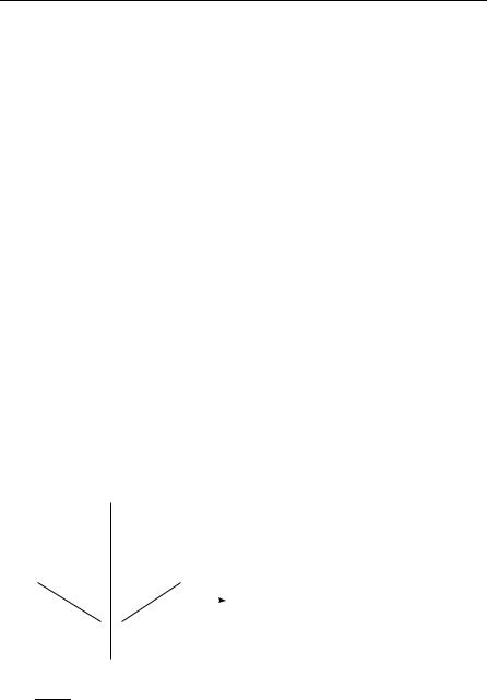
Methylene (CH2, Figure 12) is one of the rare molecules that exhibit a triplet electronic ground state. Assume we are interested in its fine-structure splitting. Apart from the ground statee X 3B1, three low-lying excited singlet

states exist: a 1A1, b 1B1, and c 1A1.

We should like to answer the following questions:

1.Is there any first-order fine-structure splitting in the electronic ground state, due to either electronic spin–orbit or spin–spin coupling?

2.Which of the excited states, a 1A1 and c 1A1, or b 1B1 is by symmetry allowed to contribute to the fine-structure splitting of X 3B1 in second order?

3.If there is a second-order spin–orbit splitting, can we predict which of the triplet sublevels is lowered in energy due to spin–orbit coupling?

For a matrix element to be nonzero, the direct products of the irreps of space and spin functions on each side have to be equal. Let us check this out first. Spatially, A1 and B1 states are involved. Table 11 presents the irreps according to which singlet and triplet spin functions transform under symmetry operations of the C2v molecular point group.

z

	H	H		Figure 12 Ground-state equilibrium struc-
				ture of methylene. The molecule is chosen
				to lie in the yz plane with z as symmetry
		y		axis. With this convention, the triplet
	C			ground state is of 3B1 symmetry. If ~x and
				~z span the molecular plane, B1 and B2 have
				to be interchanged.

dA fairly good quantum number means that coupling between states of different multiplicity is small, and the spin quantum number is close to zero (singlet), one (triplet), and so on.

eFollowing convention in spectroscopy, X labels the electronic ground state, A is the first known excited state of the same spin symmetry as X, B the second, and so on; ‘‘a’’ labels the first excited state of different spin symmetry, b the second, and so on. Symmetry labels for each state are in italics.

156 Spin–Orbit Coupling in Molecules

Table 12 Direct Product Representations for the Spatial and Spin Wave Functions of the Low-Lying Electronic States of Methylene

	Spatial	Spin
State	Symmetry	Symmetry
X 3B1	B1	A2	B2
		B1	A1
b 1B1		B2	A2
	B1	A1	B1
fa; cg 1A1	A1	A1	A1

The direct product representations of the space and spin functions are in this particular case given in Table 12. The overall symmetries of the electronic states involved tell us that there is no coupling between b 1B1 and X 3B1, whereas the 1A1 states may interact with X 3B1. However, we can give much more specific answers:

1. Concerning spin–orbit coupling, no component of the angular momentum operator is found in A1 symmetry. Therefore, there is no first-order

^	3	B1	. This statement
contribution of HSO to the fine-structure splitting of X

is true for all spatially nondegenerate electronic states.

2.On the contrary, both D2z2 x2 y2 and Dx2 y2 are totally symmetric. Hence, the triplet is split by spin–spin coupling (SSC) into three distinct multiplet levels.

3.The spatial parts of the {a, b} 1A1 states can couple to X 3B1 via the y component of the spin–orbit operator. The operator S^y couples the singlet spin function S0 (A1) to the B1 triplet function.

Summarizing, we find that spin–spin interaction is capable of splitting the ground-state triplet spin multiplet into three distinct levels. Which of the multiplet levels is lowered in energy and which is raised due to spin–spin coupling cannot be predicted by means of group theory. This raising or lowering in energy depends on the specific electronic configuration in the considered state. Among the low-lying states, only the 1A1 states are allowed to perturb the X 3B1 ground state via spin–orbit coupling. One of the triplet components (Ty) is lowered in energy due to this perturbation, the two others remain unaltered.

Linear Molecules

In systems with orbitally degenerate states, we can also exploit the Wigner–Eckart theorem for the spatial part of the wave function. Use of the WET further reduces the number of matrix elements that have to be computed explicitly.

In linear molecules or atoms where the separate projection of the total spatial and spin angular momenta on the z axis is meaningful (Russell–

Symmetry 157

Table 13 Irreps of Singlet (S) and Triplet (T) Spin Func-

~ ~

tions, the Angular Momentum Operators ( ^ and S^),

L

an Irreducible Second-Rank Tensor Operator ^ , and

D

the Position Operators ^ ^ ^ in C ðD Þ Symmetry

XYZ 1v 1h

Function/Operator

TripletMS¼0

T0

TripletMS¼ 1

T 1

Singlet

MS¼0

S0

^

^

^

^

Lz; Sz

L0;

S0

^

ð2z x y Þ=p6

0

L^

p

;

^

p

L^

1;

^

1

^

ðx iyÞ= 2

S ðx iyÞ= 2

S

^

ðxzþzx iðyzþ

ÞÞ=

D

2

2 2

D

D

zy

2

D 1

Dðx2 y2 iðxyþyxÞÞ=2

D 2

^

^

Z

p

T0

ðX iYÞ=

T 1

^

^

2

^

Irrep.

ðgÞ

ðgÞ

þðgÞðgÞ

ðgÞþðgÞ

ðgÞ

ðgÞþðuÞ

ðuÞ

Saunders coupling), ML and MS quantum numbers can be changed by the

operator ^ SO by at most one unit each, while their sum MJ has to remain con-

H

stant. Employing the nomenclature specific to linear molecules (i.e., MJ ¼ , ML ¼ , and MS ¼ ), the selection rule for spin–orbit coupling reads:

¼ 0 ¼ 0; 1 ¼ 0; 1

½189&

To determine the first-order spin–orbit splitting pattern of an orbitally degenerate electronic state, we shall make use of the energy expression obtained from the phenomenological operator, which in this case reduces to ASO because only the z component of the spin–orbit operator is involved.

Inspection of Table 13 shows that the MS ¼ 0 component of a triplet state transforms like in C1v, and the MS ¼ 1 components like the irrep. The direct product of space and spin functions is irreducible in the case of the MS ¼ 0 component. For a 3 state, the direct product results in an overall symmetry. Reduction of the direct product for MS ¼ 1 components is readily carried out and gives ¼ þ . More specifically, one obtains the splitting pattern shown in Table 14. From the entries in Table 14, we read the following results:

"First-order SOC lifts certain degeneracies but not all of them. In the particular example, the six components of a 3 state are split into

Table 14 First-Order Spin–Orbit Splitting of a 3 State

Product State

j j ¼ j þ j

E

þ1Tþ1; 1T 1

2

þ1

þASO

T ;

1

T

1

0

0

þ1p0

0

1 þ1&

SO

ð1=

Þ½ þ1

T

1

0

1

A

2

T

158Spin–Orbit Coupling in Molecules

three doubly degenerate levels. (We should point out that a degeneracy of the 0 levels is not required by group theory. The S 1Dþ2S 1 and Sþ1D 2Sþ1 components of the electronic spin–spin coupling operator and higher-order SOC lift their degeneracy. It requires a different type of interaction, that is, either the coupling to an external magnetic field or the rotation of the nuclear framework to split also the ¼ 2 and¼ 1 sublevels.)

"There is a first-order splitting pattern common to all 3 states, independent of the physical content. All the molecule-dependent

physical information is contained in the parameter ASO. These facts are, of course a consequence of the tensor properties expressed in the Wigner–Eckart theorem.

	Summary
1.	^
	Only in spatially degenerate states, HSO may cause a multiplet splitting in
	first order.
2.	^
	The operator HSO couples states of different spin and space symmetries in

second order, independent of spatial degeneracies.

3.It is possible to use the Wigner–Eckart theorem for reducing the number of matrix elements that have to be calculated. Symmetry rules can be obtained from the tensorial structure of the interaction Hamiltonians.

4.As a consequence of the WET, there is a first-order splitting pattern common to all states of a specific space þ spin symmetry, independent of the physical content.

5.Double groups: For describing the transformation properties of the a and b spin functions, it is necessary to augment the ordinary molecular point group by symmetry operations that result from multiplying the original symmetry operations by a rotation through 2p. The resulting enlarged point groups are called double groups.

6.Many-particle spin functions:

Odd number of electrons ! Fermion irreps of the double group Even number of electrons ! Boson irreps of the double group

7. Selection rules for ^ ( !: coupling allowed; n!: no interaction; u

HSO

signifies ungerade states)

a. Systems with an inversion center strictly: g !g; u !u; g n! u

b.Atoms strictly: dJJ 0 , dMJ M 0J

LS coupling: L þ L0 1 jL L0j; S0 þ S 1 jS0 Sj

c.Linear molecules strictly: ¼ 0

LS coupling: ¼ 0; 1; ¼ 0; 1; S0 þ S 1 jS0 Sj

d.Nonlinear molecules strictly: refer to direct product representations of the appropriate double group.

LS coupling: S; S0 as above

Computational Aspects

159

COMPUTATIONAL ASPECTS

General Considerations

Various approaches can be pursued to compute spin–orbit effects. Fourcomponent ab initio methods automatically include scalar and magnetic relativistic corrections, but they put high demands on computer resources. (For reviews on this subject, see, e.g., Refs. 18,19,81,82.) The following discussion focuses on two-component methods treating SOC either perturbationally or variationally. Most of these procedures start off with orbitals optimized for a spin-free Hamiltonian. Spin–orbit coupling is added then at a later stage. The latter approaches can be divided again into so-called one-step or twostep procedures as explained below.

In light molecules, SOC predominantly affects spectral properties such as fine-structure and transition probabilities. Fine-structure splittings originate both from firstand higher-order spin–orbit contributions. In the language of magnetic resonance, these are also dubbed diamagnetic and paramagnetic contributions, respectively. The latter depend both on spin–orbit coupling matrix elements and on spin-free energy differences. Independent of the spin–orbit interaction scheme, it is therefore indispensable to employ methods that take electron correlation into account.

In heavy element compounds, spin–orbit interaction is of concern also for binding energies because the mutual spin–orbit interaction between molecular states will in general be smaller than in the dissociation limit. (Sometimes this is also addressed as quenching of SOC, although the interaction does not disappear completely.) Those molecular states that correlate with the lower spin–orbit component of a heavy element atomic state will therefore be more loosely bound. In contrast, the states that dissociate to the upper atomic spin–orbit level are stabilized by SOC.

Approximately from the 3d elements onward, it is necessary to add spinindependent (scalar) relativistic corrections to the Hamiltonian.18 In early works, the differential scalar relativistic effect to molecular excitation energies was often estimated by adding mass–velocity and Darwin corrections14 perturbationally. However, even for firstand second-row transition metals, it turned out that scalar relativistic effects are preferably taken into account during the orbital optimization,83,84 whereas this is mandatory for heavier element compounds.85 In two-component methods, integrals including kinematic relativistic corrections can be generated either by utilizing relativistic effective core potentials (see, e.g., Refs. 35,37,38) or by employing a one-component relativistic all-electron Hamiltonian that is bounded from below. An overview over state-of-the-art one-component relativistic electronic structure methods has recently been given by Hess and Marian.19

Different computational strategies ought to be pursued for heavy main group elements and transition metals:

160 Spin–Orbit Coupling in Molecules

*In compounds containing heavy main group elements, electron correlation depends on the particular spin–orbit component. The jj coupled

6p1=2 and 6p3=2 orbitals of thallium, for example, exhibit very different radial amplitudes (Figure 13). As a consequence, electron correlation in the p shell, which has been computed at the spin-free level, is not transferable to the spin–orbit coupled case. This feature is named spinpolarization. It is best recovered in spin–orbit CI procedures where electron correlation and spin–orbit interaction can be treated on the same footing—in principle at least. As illustrated below, complications arise when configuration selection is necessary to reduce the size of the CI space. The relativistic contraction of the thallium 6s orbital, on the other hand, is mainly covered by scalar relativistic effects.

*The most critical part in electronic structure calculations on transition metal compounds is the determination of electron correlation at the spin-

free level. Spin–orbit coupling in open d shells can be computed very accurately by perturbational expansions.86 One reason for this behavior

lies in the fact that densities and radial expectation values of d3=2 and d5=2 orbitals do not differ dramatically. Spin-polarization effects are therefore small. Another cause is related to the length of the perturbation

expansion. In transition metal atoms, roughly speaking, only terms with equal d occupation interact via SOC. At the orbital level, an s ! d

excitation or vice versa yields spin–orbit integrals of the type hsj ^ jdi,

HSO

which are zero. As long as configurations of different d occupations do not mix extensively at the spin-free level, perturbation sums can be confined to a manifold of states with a particular d occupation.

0.56s_1/2

0.46s

6p_1/2

0.3		6p
0.2
0.1			6p_3/2
0	2	4	6	8	10
0

R (bohr)

Figure 13 Nonrelativistic 6s and 6p radial wave functions (solid) versus relativistic 6s1=2 (dotted), 6p1=2 (dashed–dotted), 6p3=2 (dashed) radial wave functions of the thallium atom calculated at the Hartree–Fock and Dirac–Fock levels, respectively.

Computational Aspects

161

*Spin-polarization should also play a minor role in lanthanides and actinides. Differential correlation between states of different f occupation and spin–orbit coupling within a given sldmf n manifold are huge,

however. Further, the number of electronic states that can be derived from an sldmf n occupation is in general too large for an explicit expansion of the spin–orbit coupled states in unperturbed ones. In spite of these difficulties, good progress has been made in recent years.56

We confine the discussion in the remainder of this section to the treatment of electronic wave functions. This confinement to electronic wave functions is justified as long as no (sharply avoided) intersystem crossings are present or other non-Born–Oppenheimer effects such as rovibronic (rotational/vibrational/electronic) coupling are involved. Intersystem crossings will be discussed in connection to nonradiative transitions.

Evaluation of Spin–Orbit Integrals

Early implementations of Breit-Pauli spin–orbit integrals were based on Slater-type orbitals (STOs).63,87–90 All these programs involve numerical inte-

gration schemes that become prohibitively expensive in polyatomic molecules. Kern and Karplus91 proposed a Gaussian transform for STOs, but explicit formulas were only given for s functions. For a while, Gaussian lobe functions were popular because they are composed only of s functions.92–94 Besides s orbitals, p orbitals are easily described by linear combinations of lobe functions, but the extension to higher angular momentum basis functions leads to numerical problems. King and Furlani95 derived formulas for evaluating Breit-Pauli (BP) integrals in the basis of Cartesian Gaussians numerically by means of Rys quadrature techniques.

Actual computer codes for polyatomic molecules employ either Cartesian or Hermite Gaussian functions. The calculation of all-electron spin–orbit integrals makes use of second derivatives of Coulomb integrals with respect to nuclear coordinates.93,96–104 The relation between Coulomb and BP spin–obit integrals is immediately apparent, if the BP operator is written as in expressions [101] and [102]. Instead of acting with r on 1=^r in integrals of rð1=^rÞ r, the r on the left can be applied to the bra vector and the other one to the ket vector. The derivative of an s function is a p function; taking the derivative of a p function yields an s and a d function, and so on. In this way, the spatial parts of a BP integral can be written as a linear combination of Coulomb integrals.

The no-pair spin–orbit Hamiltonian [105] differs from the correspond-

							^	^
ing2 BP terms [103] by			momentum dependent factors of the type A					i=ðEi þ
			2	^	^	^
mc Þ or	^ ^	^					have been	defined
	ðAiAjÞ=ðEi þ mec Þ, where			Ei	and Ai	or Aj

in [106] and [107], respectively. There are essentially two ways of taking these factors into account.

162 Spin–Orbit Coupling in Molecules

*The first was pioneered by Samzow et al.103 and makes use of a method proposed by Hess for spin-independent one-electron no-pair operators.25 This approach resembles a resolution-of-the-identity ansatz. As the kinematical factors are functions of the momentum, they are most easily evaluated in momentum space. The auxiliary basis set should span the momentum space as completely as possible. If the set of uncontracted functions is not sufficient for this purpose, it has to be augmented by further primitives. First, the spatial auxiliary basis functions are orthogonalized. The matrix of the nonrelativistic kinetic energy operator

p^2i =2me is diagonalized in a second step. Its eigenvectors form a discrete representation of the (continuous) spectrum of the momentum operator. If the basis were complete, then every other operator that can be written as a polynomial of the momentum would be diagonal. In a finite basis, this property is only approximately fulfilled. The eigenvectors of the kinetic energy matrix are utilized to evaluate the momentum dependent factors in the no-pair Hamiltonian. The last step is a transformation back to the original auxiliary basis.

*The second way avoids transformations back and forth, which are

particularly time consuming for two-electron integrals. Almlo¨ f and

co-workers

105

^

^

m

c

2

or

noticed that kinematical factors such as A

i=ð

E

i þ

Þ

^ ^

^

2

e

ðAiAjÞ=ðEi þ mec

Þ can be turned over to the basis functions instead of

applying them to the BP operator. Under certain circumstances, the modified basis functions can be reexpanded in the original basis so that only the contraction coefficients change. In this way, any program that evaluates BP integrals can be utilized to compute approximate no-pair integrals.

Effective core-potential [127] and atomic mean-field spin–orbit operators [128] are in essence one-center operators. Only the projectors contain multicenter terms, but these yield merely overlap integrals. One-center spin– orbit integrals are therefore most easily evaluated in the basis of spherical Gaussians.64 The computation reduces then to a 1D radial integration and multiplication by analytically determined factors from the angular part. Exploiting the spherical symmetry of the one-center terms thus appreciably speeds up the integral evaluation time and appears to be the only tractable way to perform all-electron spin–orbit calculations in large molecules. For further usage in a molecular code, a basis set transformation to a Cartesian or so-called real spherical Gaussian basis is performed.f Atomic mean-field

fReal spherical Gaussian basis functions are not proper ^ eigenfunctions. They are linear

‘z

combinations of spherical Gaussians expð ar2Þ ðamYm‘ þ b mY‘ mÞ with coefficients am and b m chosen such that real basis functions result.

Computational Aspects

163

integrals for ab initio model potentials (AIMPs) are evaluated in an all-electron basis first and are transferred then to the AIMP basis.65 A prerequisite for this procedure to work is an approximate matching of the respective valence orbital exponents and contraction coefficients. Therefore, this approach should

only be applied in connection with generalized contracted basis sets of the Raffenetti or atomic natural orbital types.106,107

Perturbational Approaches to Spin–Orbit Coupling

As in all perturbational approaches, the Hamiltonian is divided into an unperturbed part Hð0Þ and a perturbation V. The operator Hð0Þ is a spin-free, one-component Hamiltonian and the spin–orbit coupling operator takes the role of the perturbation. There is no natural perturbation parameter l in

this particular case. Instead, ^ is assumed to represent a first-order pertur-

HSO

bation Hð1Þ. The perturbational treatment of fine structure is an inherent twostep approach. It starts with the computation of correlated wave functions and energies for pure spin states—mostly at the CI level. In a second step, spin– orbit perturbed energies and wavefunctions are determined.

Rayleigh–Schro¨ dinger Expansion

In Rayleigh–Schro¨ dinger perturbation theory, perturbed wave functions are expanded in the infinite set of eigenfunctions ð0Þ of the unperturbed Hamiltonian. In practical applications, the sum over states is truncated to a finite number, of course. In principle, the eigenstates ð0Þ could be constructed from determinants using separate sets of molecular orbitals. Mutually nonorthogonal orbital bases add a complication to the evaluation of matrix elements, in particular for two-electron operators, as the Slater–Condon rules [119] and [120] are not applicable right away. Formulas for self-consistent field wave functions have been worked out by Bearpark et al.104 These involve bi-orthogonalization of the orbital sets and cofactors resulting from nonunity overlaps. Employing different orbitals for different states (DODS) is desirable in many cases and certainly yields more accurate excitation energies than the use of a common set of molecular orbitals (MOs), but the evaluation of spin– orbit matrix elements for general CI expansions is prohibitively expensive. In most cases, a common set of MOs is used as a one-particle basis for the construction of the determinants. Further, the order of the perturbation expansion is often confined to second order in the energy and to first order in the wave function.

A first-order contribution to the energy is obtained only for spatially degenerate states. Let us assume that the unperturbed state j ðk0Þi has a d-fold degenerate eigenvalue, including both spin and space degeneracies. According to the rules of degenerate perturbation theory, the first-order