Berrar D. et al. - Practical Approach to Microarray Data Analysis

4 Chapter 1

A natural error is to suppose that, once the genome is known, everything important in human biology is understood. This is far from the truth. As an analogy: suppose we have obtained a catalogue of all the 40,000-odd parts and tools needed to make an automobile; do we then understand its design, can we improve it? Not if the catalogue is like the human genome, with entries mostly in random order, with no indication of which tool is needed for fitting which part, or where the parts go, or which has to be connected to what, or how many of each we need. And imagine that (as experience teaches us is true for the genome) that many catalogue entries may be ambiguous, so that the same part number can describe a range of more or less related parts. Still worse; many parts, as specified in the catalogue, don’t actually fit, and have to be machined down or have holes drilled through them or small attachments stuck onto them before they can be used at all. Add that some entries in the catalogue are for parts that aren’t used any longer, or are unusable...

All that analogy is true for the proteins encoded by the genome. Proteins are the ultimate product of the gene expression process. All the proteins synthesized from a cell’s genome constitute its proteome. Chemically, proteins are polymers that are formed from 20 different subunits called amino acids. The linear chain of amino acids making up a protein, dictated by the sequence of bases in the mRNA, is known as its primary structure or sequence. Within its normal physiological environment, an amino acid sequence assumes a three-dimensional conformation, which is the major determinant of the protein’s biological function. For each amino acid sequence, there is a stable three-dimensional structure sometimes referred to as the protein’s native state; many proteins have a range of possible native states, and can switch between them according to their interactions with other molecules. The native state of a protein and the folding process involved in reaching this state from its initial linear orientation are dictated by the primary sequence of the protein. Despite the strong deterministic correspondence between the primary sequence and the native state of a protein, the processes involved in protein folding are highly complex and difficult to capture and describe logically. Protein folding and structure prediction have been the subjects of ongoing research for some time.

In many ways, proteins can be considered as the biochemical “workhorses” of an organism. Proteins play a variety of roles in life processes, ranging from structural (e.g., skin, cytoskeleton) to catalytic (enzymes) proteins, to proteins involved in transport (e.g., haemoglobin), and regulatory processes (e.g., hormones, receptor/signal transduction), and to proteins controlling genetic transcription and the proteins of the immune system. Given their importance in terms of biological function, it is no surprise that many applications in biotechnology are directly related to the

1. Introduction to Microarray Data Analysis

5

understanding of protein structure and function. This is perhaps most impressively demonstrated by modern drug development. The principal working mechanism of most known drugs is based on the idea of selectively modifying (by interaction) the function of a protein to affect the symptoms or underlying causes of a disease. Typical target proteins of most existing drugs include receptors, enzymes, and hormones. Therefore, many experts foresee proteomics, the study of structure and function of proteins, as the next big step in biomolecular research.

In many biomolecular studies, the most important issue is to measure real gene expression, that is the abundance of proteins. However, as we will see in more detail below, DNA microarray experiments do measure the abundance of mRNA, but not protein abundance. According to a simple, traditional view of gene expression, there is a direct one-to-one mapping from DNA to mRNA to protein. To put it another way, a specific gene (i.e. genomic DNA sequence) will always produce one and the same amino acid sequence of the corresponding protein, which will then fold to assume its native state. Given this simplified scheme, measuring mRNA abundance would provide us with highly accurate information on protein abundance, as protein and mRNA abundance are proportional due to the direct mapping. We would also know the primary structure of the proteins corresponding to the measured mRNA, since the genetic code allows us to deduce the amino acid sequence from a given DNA or RNA sequence. Unfortunately, gene expression is in reality more complex.

The modern view of gene expression paints a more intricate picture, which suggests a highly dynamic gene expression scenario. There are various ways in which proteins are formed and modified; and indeed, the genome itself is subject to alterations.

First, genomic DNA itself may undergo changes, as a result of the replication machinery making mistakes, or attempting to copy damaged DNA and getting it wrong. DNA bases can be changed; small or large regions can be inserted or deleted or duplicated, pieces of one DNA molecule can be joined onto pieces of another, RNA can be copied backwards into DNA (reverse transcription), regions of junk DNA derived from viruses can jump about the genome.

Second, the (forward) transcription process is more complicated. One gene may be transcribed to give a range of possible products. When composing the final mRNA sequence, the transcription process uses a mechanism called splicing to cut out some regions (introns), so that only the remaining segments (exons) survive to be translated to protein. This process may yield alternative versions of mRNA sequences due to alternative splicing. A region of mRNA that in one case is treated as intron/exon/intron may in another be treated as one large intron; a gene coding for 3 possible

6 Chapter 1

introns, A, B and C can thus produce a mRNA with an ABC sequence, or alternatively just AC. (With multiple introns, much greater permutations are of course possible. The current record is held by a gene expressed in the brain of the fruitfly Drosophila, which could in principle be alternatively spliced in over 40,000 different ways)

Another source of variation comes from promoter choice. A promoter is a specific location or site where the transcription of a gene from DNA to mRNA begins. Genes may have multiple promoters, thus giving rise to different transcript versions and hence different proteins even without alternative splicing

It is also possible – some cases are known, and we do not know how many there are – for an mRNA to be “edited” before it is translated. One base in the mRNA can be replaced by another, altering one amino acid (or, drastically, converting a signal for an amino acid into a signal to stop translating early).

Furthermore, there is no necessary connection between the amount of an mRNA present (in whatever spliced or edited form) and the amount of protein translated from it. There is, in a general sort of way, a correlation between mRNA abundance and the corresponding protein abundance, but there is no doubt that rates of translation can be differentially controlled.

Lastly, there are post-translational modifications. These are structuremodifying alterations occurring after the translation process. Proteins may be split up into smaller fragments, or have their ends or internal regions removed; amino acids may be altered by adding (temporarily or permanently) other chemical groups to them, sometimes with drastic effects on the protein’s catalytic or structural properties.

With all these caveats, we should stress that although DNA gene microarrays are often thought of as instruments for measuring gene expression, what they really measure is mRNA transcript abundances. They do not always distinguish between different forms of processed mRNA, and they can give no information about differential translation rates, nor about post-translational modification. But they do give some valuable information, quickly and fairly easily. One of the main reasons why researchers are pursuing DNA microarray studies with such intensity, in the full knowledge of their limitations, is the fact that protein expression and modification studies are still very expensive, and often involve highly specialized and delicate techniques, (e.g., 2D-gel electrophoresis, mass spectrometry). Highthroughput protein-detecting arrays or chips are beginning to emerge; however, there are still a number of issues to be resolved before this technology is mature. Critical issues involve efficient methods for largescale separation and purification of proteins, and the maintenance of the active biological configuration of proteins while they are attached to the

1. Introduction to Microarray Data Analysis

7

surface of a chip. So at the present time, and for the immediately foreseeable future, DNA microarray technology constitutes a useful compromise for carrying out explorative high-throughput experiments. Because of the inherent limitations, one should exercise extreme caution when interpreting the results of such microarray experiments, even if their analysis is perfect.

The biochemical details of gene expression are highly intricate. Many good texts exist on this subject, for example, Schena et al., 1995; Raskó and Downes, 1995.

2.2Brewing up the Hybridization Soup

To summarize the last section: a great deal of modern molecular biology revolves around nucleotide polymers – DNA and RNA – and amino acid polymers, proteins. DNA microarrays measure a cell’s transcript via the abundance of mRNA molecules, but not protein concentrations. This section will illustrate the biochemical principles involved in measuring transcripts with microarrays.

A number of techniques have been developed for measuring gene expression levels, including northern blots, differential display, and serial analysis of gene expression. DNA and oligonucleotide microarrays are the latest in this line of methods. They facilitate the study of expression levels in parallel (Duggan et al., 1999). All these techniques exploit a potent feature of the DNA duplex – the sequence complementarity of the two strands. This feature makes hybridization possible. Hybridization is a chemical reaction in which single-stranded DNA or RNA molecules combine to form doublestranded complexes (see schematic illustration in Figure 1.1). The famous DNA double helix is an example of such a molecular structure.

The hybridization process is governed by the base-pairing rules: specific bases in different strands form hydrogen bonds with each other. For DNA

8 Chapter 1

the matching pairs are adenine-thymine and cytosine-guanine. Hybridization is a nonlinear reaction. Yield – the number or concentration of nucleic acid elements binding with each other in the resulting double-stranded molecule

– depends critically on the concentration of the original single-stranded polymers and on how well their sequences align or match. It is this yield that is measured in a microarray experiment.

Before we proceed to an actual hypothetical microarray experiment, let us look at color-coded genes (green and red ones) in competitive and comparative hybridization. In order to selectively detect and measure the amount of mRNA that is contained in an investigated sample, we must label the mRNA with reporter molecules. The reporters currently used in microarray experiments include fluorescent dyes (fluors), for example, cyanine 3 (Cy3) and cyanine 5 (Cy5).

Let us assume we have two samples of transcribed mRNA from two different sources, sample 1 and sample 2. Both samples may consist of multiple copies of many genes. We have also a probe, which is a specific nucleic acid sequence, perhaps a gene, or a characteristic subsequence of a gene, or a short, artificially composed nucleotide sequence. Like the two samples, the probe will contain many copies of the sequence in question. This is important because sufficient amounts are needed to get the hybridization reaction going, and to be able to detect and measure the various concentrations. What we want to find out is the relative abundance of the mRNA complementary to the probe sequence within sample 1 and sample 2. Sample 1, for example, may contain three times as many copies of sequences complementary to the probe as sample 2, or they may not be contained in either sample at all. To find out the exact answer, we proceed as follows (see also Figure 1.2):

1.Prepare a mixture consisting of identical probe sequences. In this scheme of things the probe is a kind of “sitting duck”, awaiting hybridization.

2.Label sample 1 with green-dyed reporter.

3.Label sample 2 with red-dyed reporter.

4.Simultaneously give both sample mixtures the chance to hybridize with the probe mixture. Here, sample 1 and sample 2 are said to compete with each other in an attempt to hybridize with the probe.

5.Gently stir for five minutes.

6.Filter the mixture to retain only those probe sequences that have hybridized, that is, formed a double-stranded polymer.

1. Introduction to Microarray Data Analysis

9

7.Measure the amount or intensity of green and red in the filtered mixture, and compare the amounts to determine the relative abundance of the probe sequence.

8.Jot down the result, add a little salt, and enjoy.

2.3What You Always Wanted to know About Gene X

This section briefly looks at a hypothetical DNA microarray experiment and the various steps involved. However, for reasons of illustration this experiment is dealing with a rudimentary array consisting of only four genes rather than hundreds or thousands commonly used in such experiments. Notice, that because of RNA’s inherent chemical instability, it is often useful to work with a more stable complementary DNA (cDNA) made by reverse transcription, rather than with mRNA, at intermediate steps. However, before the array is made, the cDNA is denatured (broken up into its individual strands) to allow the hybridization reaction.

Typical goals of DNA microarray experiments involve the comparison of gene transcription (expression) in two or more kinds of cells (e.g., cardiac muscle versus prostate epithelium), and in cells exposed to different conditions, for example, physical (e.g., temperature, radiation), chemical (e.g., environmental toxins), and biological conditions (e.g., normal versus disease, changing nutrient availability, cell cycle variations, drug response). Genetic diseases like cancer are characterized by genes being inappropriately transcribed, or missing altogether. A cDNA microarray study can pinpoint the transcription differences between normal and diseased, or it can reveal different patterns of abnormal transcription to identify different disease variations or stages.

10

Chapter 1

Let us imagine a study involving ten human patients with two different forms of the same type of cancer; six patients suffer from form A and four from form B. Further, let us assume that we want to investigate four different genes, a, b, c, and d, and their roles in the disease. To help us answer this question we set up a cDNA microarray experiment. Initially, we would hope to find characteristic expression patterns, which would help us to formulate more specific hypotheses. Clearly, in a more realistic scenario, we would like to analyze many more genes at the same time. But for the sake of this illustration, we are just looking at four genes. The following outlines the various steps we need to take care of for this experiments (see also Figure 1.3).

1.Probe preparation. Prepare one DNA microarray per patient, using a standard DNA (possibly cDNA).

2.Target sample preparation. Obtain, purify, and dye target mRNA samples.

3.Reference sample preparation. Obtain and prepare reference or control mRNA and label it.

4.Competitive hybridization. Hybridize target and reference mRNA with the cDNA on the array.

5.Wash up the dishes.

6.Detect red-green intensities. Scan the array to determine how much target and reference mRNA is bound to each spot.

7.Determine and record relative mRNA abundances.

The probe preparation step involves the manufacturing of sufficient amounts of cDNA sequences that are identical to the sequence of the studied genes. In place of the full sequence, it is often more practical to use a characteristic subset with 500 to 2,500 nucleotides in length. The cDNA sequence mixtures representing the investigated genes are then affixed to the array (a kind of glass slide). Normally, the mixtures are placed as round spots on the array and arranged in a grid-like fashion, hence the name microarray. At least for larger experiments, we would like to record information about where on the array which gene is placed so that we can later track the right data. In addition, we would record any information relevant to the genes in question, for example, the precise nucleotide sequence, known biological function, pointers to relevant literature, and so on.

1. Introduction to Microarray Data Analysis

11

Target refers to the actual entities or samples we want to measure: in this case, the transcribed mRNA from tissue or serum cells of our patients. First, we must obtain the tissue or serum cells. Once the cells are at hand, mRNA must be extracted from the cells, purified, dyed (i.e. labeled with reporter molecules), and converted into a suitable chemical RNA form. In the diagram of Figure 1.3 we label the target sample with “red” dye and the reference with green “dye”. The colors red and green are arbitrary. It does not necessarily imply that the actual reporter molecules are indeed red or green. However, we use these colors here, since in the final digitized, falsecolor graphics image, the color red is chosen to represent target mRNA abundance and green for reference abundance.

The reference sample is used as a baseline relative to which we measure the abundance of target mRNA. There are two common choices for references samples: standard reference and control. Standard references (also called universal references) are often derived from mRNA pools unrelated to the target samples of the experiment. Standard references should contain sufficient amounts of mRNA from the genes studied with the array. So for our four-gene example, we could use a standard reference from which we know that it contains “standard” mRNA of the four genes a, b, c, and d. Control samples are also employed as references. In contrast to references, controls are somehow related to the experiment at hand. For example, in a normal-versus-disease study, the control may represent tissue from the normals. Once sufficient amounts of reference mRNA is produced, it is labeled with reporters. Clearly, the reporter molecules used here must be such that we can later distinguish between reference from target mRNA. In the four-gene example, we dye the reference sample green.

12 Chapter 1

Now we are ready for hybridization between the labeled target and reference mixtures. We pour on the mixtures, and let them hybridize to the array.

Once the hybridization reaction is completed, we wash off any reference and target material that has not managed to find a probe partner. This leaves us with the array depicted in the right part of Figure 1.3. When you step back far enough from the book, you will recognize that the spot labeled a is dark, the one labeled c is bright, whereas the two other spots (labeled b and d) appear gray. Performing a suitable color conversion in your head, you will, after a while, be able to see a red, a green, and two orange spots on our fourgene array. Get the picture? Basically, what this tells us is that (a) gene a is much more active (highly expressed) in the target than in the standard or reference sample, as the red-dyed mRNA sequences have massively outperformed the green-dyed sequences in hybridizing to probe sequences representing gene a. By a similar argument, we can say (b) that gene c of the target sample is underexpressed when compared to the standard reference, and (c) that both the expression of gene b and d seems balanced, that is, the transcript mRNA abundance in the target is roughly the same as that in the reference. Hence, we get orange.

In real microarray experiments, it is impractical, if not impossible, to determine the relative mRNA abundances with the naked eye. To detect and measure the relative abundances of reference and target material, we use a device equipped with a laser and a microscope. The fluorescent reporter molecules with which we have labeled the samples emit detectable light of a particular wavelength when stimulated by a laser. The intensity of the emitted light allows us to estimate quantitatively the relative abundances of transcribed mRNA. After the scanning we are left with a high-resolution, false-color digital image. Image analysis software takes over here to derive the actual numerical estimates for the measured expression levels (Yang et al., 2000). These numbers may represent absolute levels or ratios, reflecting the target’s expression level against that of the reference.

As far as our four-gene experiment is concerned, we stick with ratio measures. For example, for patient 1 of our study, we may have obtained the following expression ratios: r(a) = 5.00, r(b) = 0.98, r(c) = 0.33, and r(d) = 0.89. In this scheme, a value close to 1.00 means balanced expression, 2.00 means the target mRNA abundance is two times as high as that in the reference, and 0.50 means the reference abundance is twice as high as that of the target.

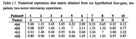
To complete our four-gene, ten-patient experiment, we must repeat the entire procedure ten times, and produce one array per patient. Once all arrays are done, we derive, record, and integrate the expression profiles of all patients in a single data matrix along with other information needed to analyze the data. Table 1.1 illustrates such data in the context of the four-

1. Introduction to Microarray Data Analysis

13

gene example expression study. Notice, the data in Table 1.1 is not normalized and no specific data transformations have been carried out.

Each numbered column in Table 1.1 holds the data related to a particular patient: patient identifier, tumor type, and the measured expression levels of the four studied genes. In a real experiment, the generated data matrix would of course be more complex (many more genes and more patients) and perhaps include also clinical data and information on the studied genes. However, the data table as depicted illustrates how the data from multiple arrays can be integrated along with other information so as to facilitate further processing. Owing to the small scale (four genes, ten patients) of our experiment and the deliberate choice of expression levels, we are able to analyze the data qualitatively by visual inspection.

First, we observe that there are no recorded expression values (depicted by question mark) for patient 5 and gene b, and for patient 8 and gene c. There may be many reasons why these values are missing. Numerous techniques exist to deal with missing values at the data analysis stage.

Second, for tumor A patients the expression levels of gene a seem to have a tendency to be by a factor 2 or more higher than the base line level of 1.00. At the same time, for tumor B patients, a’s expression levels tend to be a factor two or more lower than the reference level. This differential expression pattern of gene a suggests that the gene may be involved in the events deciding the destiny of the tumor cell in terms of developing into either of the two forms. If this difference is statistically significant on a particular confidence level remains to be seen.

Third, there seems to be also a differential expression pattern for gene c. However, here we observe the tendency to underexpressed levels for tumor A and overexpressed for tumor B.

Fourth, most expression values of gene b and d appear to be “hovering” about the base line of 1.00, suggesting that the two genes are not differentially expressed across the studied tumors.

Fifth, we observe that high expression levels of gene a are often matched by a low level of gene c for the same patient, and vice versa. This suggests that the two genes are (negatively) co-regulated.