Mankiw Macroeconomics (5th ed)

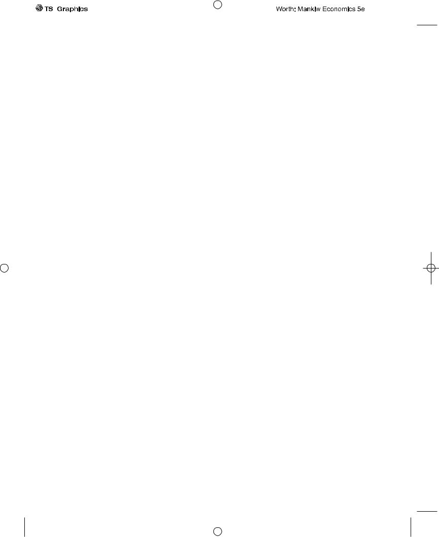
User SONPR:Job EFF01417:6264_ch01:Pg 0:23907#/eps at 100% *23907*										Fri, Nov 9, 2001 11:52 AM

part I

Introduction

User SONPR:Job EFF01417:6264_ch01:Pg 1:21266#/eps at 100% *21266*				Fri, Nov 9, 2001 11:52 AM

C H A P T1E R O N E

The Science of Macroeconomics

The whole of science is nothing more than the refinement of everyday

thinking.

— Albert Einstein

1-1 What Macroeconomists Study

Why have some countries experienced rapid growth in incomes over the past century while others stay mired in poverty? Why do some countries have high rates of inflation while others maintain stable prices? Why do all countries experience recessions and depressions—recurrent periods of falling incomes and rising unemployment—and how can government policy reduce the frequency and severity of these episodes? Macroeconomics, the study of the economy as a whole, attempts to answer these and many related questions.

To appreciate the importance of macroeconomics, you need only read the newspaper or listen to the news. Every day you can see headlines such as INCOME GROWTH SLOWS, FED MOVES TO COMBAT INFLATION, or STOCKS FALL AMID RECESSION FEARS. Although these macroeconomic events may seem abstract, they touch all of our lives. Business executives forecasting the demand for their products must guess how fast consumers’ incomes will grow. Senior citizens living on fixed incomes wonder how fast prices will rise. Recent college graduates looking for jobs hope that the economy will boom and that firms will be hiring.

Because the state of the economy affects everyone, macroeconomic issues play a central role in political debate.Voters are aware of how the economy is doing, and they know that government policy can affect the economy in powerful ways.As a result, the popularity of the incumbent president rises when the economy is doing well and falls when it is doing poorly.

Macroeconomic issues are also at the center of world politics. In recent years, Europe has moved toward a common currency, many Asian countries have experienced financial turmoil and capital flight, and the United States has financed large trade deficits by borrowing from abroad. When world leaders meet, these topics are often high on their agendas.

2 |

User SONPR:Job EFF01417:6264_ch01:Pg 2:24475#/eps at 100% *24475*				Fri, Nov 9, 2001 11:52 AM

C H A P T E R 1 The Science of Macroeconomics | 3

Although the job of making economic policy falls to world leaders, the job of explaining how the economy as a whole works falls to macroeconomists.Toward this end, macroeconomists collect data on incomes, prices, unemployment, and many other variables from different time periods and different countries. They then attempt to formulate general theories that help to explain these data. Like astronomers studying the evolution of stars or biologists studying the evolution of species, macroeconomists cannot conduct controlled experiments. Instead, they must make use of the data that history gives them. Macroeconomists observe that economies differ from one another and that they change over time. These observations provide both the motivation for developing macroeconomic theories and the data for testing them.

To be sure, macroeconomics is a young and imperfect science. The macroeconomist’s ability to predict the future course of economic events is no better than the meteorologist’s ability to predict next month’s weather. But, as you will see, macroeconomists do know quite a lot about how the economy works.This knowledge is useful both for explaining economic events and for formulating economic policy.

Every era has its own economic problems. In the 1970s, Presidents Richard Nixon, Gerald Ford, and Jimmy Carter all wrestled in vain with a rising rate of inflation. In the 1980s, inflation subsided, but Presidents Ronald Reagan and George Bush presided over large federal budget deficits. In the 1990s, with President Bill Clinton in the Oval Office, the budget deficit shrank and even turned into a budget surplus, but federal taxes as a share of national income reached a historic high. So it was no surprise that when President George W. Bush moved into the White House in 2001, he put a tax cut high on his agenda. The basic principles of macroeconomics do not change from decade to decade, but the macroeconomist must apply these principles with flexibility and creativity to meet changing circumstances.

C A S E S T U D Y

The Historical Performance of the U.S. Economy

Economists use many types of data to measure the performance of an economy. Three macroeconomic variables are especially important: real gross domestic product (GDP), the inflation rate, and the unemployment rate. Real GDP measures the total income of everyone in the economy (adjusted for the level of prices).The inflation rate measures how fast prices are rising.The unemployment rate measures the fraction of the labor force that is out of work. Macroeconomists study how these variables are determined, why they change over time, and how they interact with one another.

Figure 1-1 shows real GDP per person in the United States. Two aspects of this figure are noteworthy. First, real GDP grows over time. Real GDP per person is today about five times its level in 1900.This growth in average

User SONPR:Job EFF01417:6264_ch01:Pg 3:24476#/eps at 100% *24476*				Fri, Nov 9, 2001 11:52 AM

4 |	P A R T	I	Introduction
		f i g u r e		1 - 1
		Real GDP per person											First oil price shock
		(1996 dollars)			World		Great		World Korean		Vietnam		Second oil price shock
				35,000
					War I		Depression		War II	War		War
				30,000
				20,000
				10,000
				5,000
				3,000	1910	1920	1930	1940		1950	1960	1970	1980	1990	2000
				1900
															Year

Real GDP per Person in the U.S. Economy

Real GDP measures the total income of everyone in the economy, and real GDP per person measures the income of the average person in the economy. This figure shows that real GDP per person tends to grow over time and that this normal growth is sometimes interrupted by periods of declining income, called recessions or depressions.

Note: Real GDP is plotted here on a logarithmic scale. On such a scale, equal distances on the vertical axis represent equal percentage changes. Thus, the distance between $5,000 and $10,000 (a 100 percent change) is the same as the distance between $10,000 and $20,000 (a 100 percent change).

Source: U.S. Bureau of the Census (Historical Statistics of the United States: Colonial Times to 1970) and U.S. Department of Commerce.

income allows us to enjoy a higher standard of living than our great-grand- parents did. Second, although real GDP rises in most years, this growth is not steady. There are repeated periods during which real GDP falls, the most dramatic instance being the early 1930s. Such periods are called recessions if they are mild and depressions if they are more severe. Not surprisingly, periods of declining income are associated with substantial economic hardship.

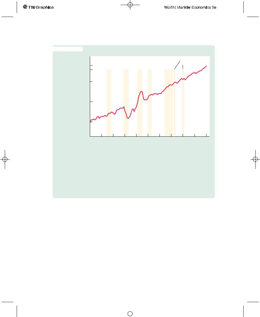
Figure 1-2 shows the U.S. inflation rate. You can see that inflation varies substantially. In the first half of the twentieth century, the inflation rate averaged only slightly above zero. Periods of falling prices, called deflation, were almost as common as periods of rising prices. In the past half century, inflation has been the norm.The inflation problem became most severe during the late 1970s, when prices rose at a rate of almost 10 percent per year. In recent years,

User SONPR:Job EFF01417:6264_ch01:Pg 4:24477#/eps at 100% *24477*				Fri, Nov 9, 2001 11:52 AM

					C H A P T E R 1			The Science of Macroeconomics | 5
f i g u r e	1 - 2
	Percent
	30		World	Great	World	Korean		Vietnam	First oil price shock
									Second oil price shock
	25		War I	Depression	War II	War		War
	20
Inflation	15
	10
	5
	0
	−5
Deflation	−10
	−15
	−20	1910	1920	1930	1940	1950	1960	1970	1980	1990	2000
	1900
											Year

The Inflation Rate in the U.S. Economy

The inflation rate measures the percentage change in the average level of prices from the year before. When the inflation rate is above zero, prices are rising. When it is below zero, prices are falling. If the inflation rate declines but remains positive, prices are rising but at a slower rate.

Note: The inflation rate is measured here using the GDP deflator.

Source: U.S. Bureau of the Census (Historical Statistics of the United States: Colonial Times to 1970) and U.S. Department of Commerce.

the inflation rate has been about 2 or 3 percent per year, indicating that prices have been fairly stable.

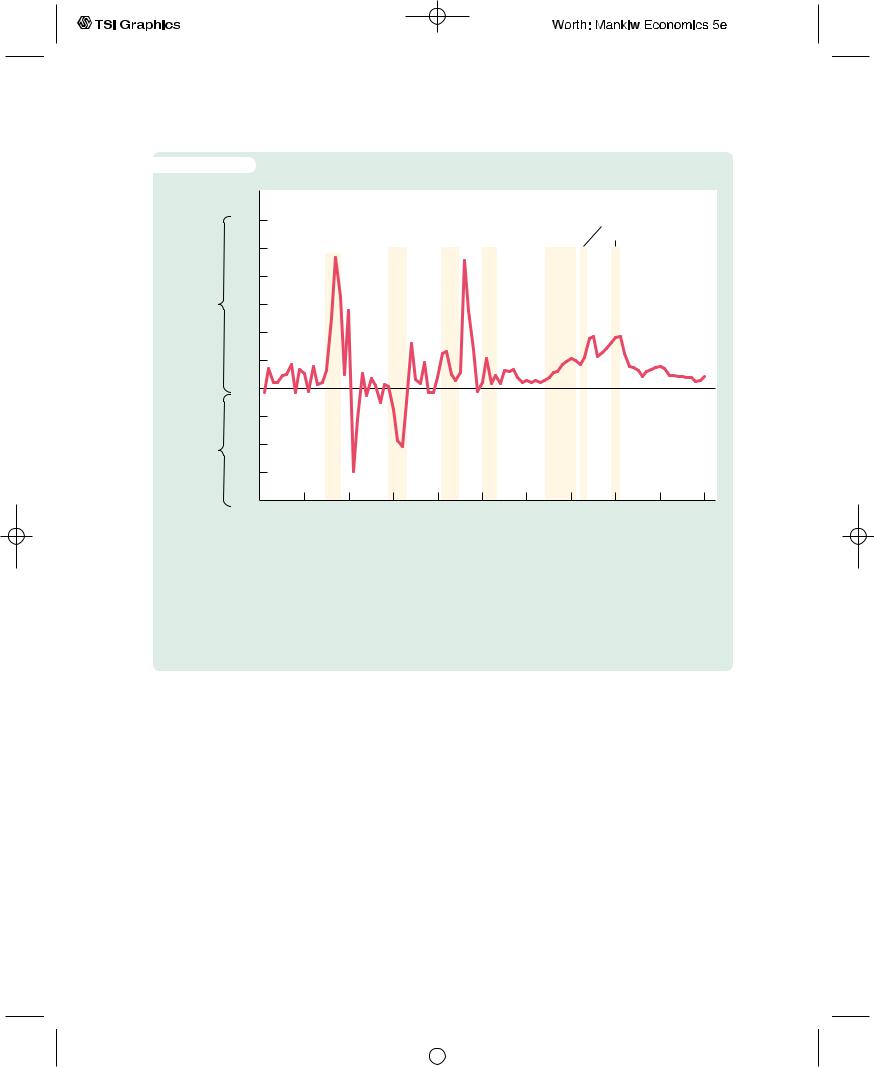
Figure 1-3 shows the U.S. unemployment rate. Notice that there is always some unemployment in our economy. In addition, although there is no longterm trend, the amount of unemployment varies from year to year. Recessions and depressions are associated with unusually high unemployment.The highest rates of unemployment were reached during the Great Depression of the 1930s.

These three figures offer a glimpse at the history of the U.S. economy. In the chapters that follow, we first discuss how these variables are measured and then develop theories to explain how they behave.

User SONPR:Job EFF01417:6264_ch01:Pg 5:24478#/eps at 100% *24478*				Fri, Nov 9, 2001 11:52 AM

6 |	P A R T I	Introduction
	f i g u r e		1 - 3
	Percent										First oil price shock
	unemployed				World	Great	World	Korean		Vietnam
					War I	Depression	War II	War		War	Second oil price shock
			25
			20
			15
			10
			5
			0	1910	1920	1930	1940	1950	1960	1970	1980	1990	2000
			1900
													Year

The Unemployment Rate in the U.S. Economy

The unemployment rate measures the percentage of people in the labor force who do not have jobs. This figure shows that the economy always has some unemployment and that the amount fluctuates from year to year.

Source: U.S. Bureau of the Census (Historical Statistics of the United States: Colonial Times to 1970) and U.S. Department of Commerce.

1-2 How Economists Think

Although economists often study politically charged issues, they try to address these issues with a scientist’s objectivity. Like any science, economics has its own set of tools—terminology, data, and a way of thinking—that can seem foreign and arcane to the layman.The best way to become familiar with these tools is to practice using them, and this book will afford you ample opportunity to do so.To make these tools less forbidding, however, let’s discuss a few of them here.

Theory as Model Building

Young children learn much about the world around them by playing with toy versions of real objects. For instance, they often put together models of cars, trains, or planes.These models are far from realistic, but the model-builder learns

User SONPR:Job EFF01417:6264_ch01:Pg 6:24479#/eps at 100% *24479*				Fri, Nov 9, 2001 11:52 AM

C H A P T E R 1 The Science of Macroeconomics | 7

a lot from them nonetheless.The model illustrates the essence of the real object it is designed to resemble.

Economists also use models to understand the world, but an economist’s model is more likely to be made of symbols and equations than plastic and glue. Economists build their “toy economies” to help explain economic variables, such as GDP, inflation, and unemployment. Economic models illustrate, often in mathematical terms, the relationships among the variables. They are useful because they help us to dispense with irrelevant details and to focus on important connections.

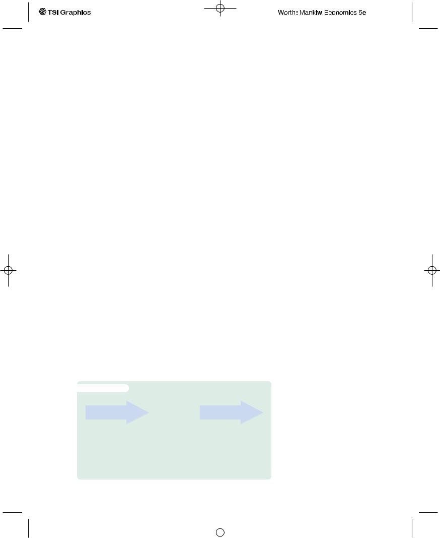
Models have two kinds of variables: endogenous variables and exogenous variables. Endogenous variables are those variables that a model tries to explain. Exogenous variables are those variables that a model takes as given.The purpose of a model is to show how the exogenous variables affect the endogenous variables. In other words, as Figure 1-4 illustrates, exogenous variables come from outside the model and serve as the model’s input, whereas endogenous variables are determined inside the model and are the model’s output.

To make these ideas more concrete, let’s review the most celebrated of all economic models—the model of supply and demand. Imagine that an economist were interested in figuring out what factors influence the price of pizza and the quantity of pizza sold. He or she would develop a model that described the behavior of pizza buyers, the behavior of pizza sellers, and their interaction in the market for pizza. For example, the economist supposes that the quantity of pizza demanded by consumers Qd depends on the price of pizza P and on aggregate income Y.This relationship is expressed in the equation

Qd = D(P, Y),

where D( ) represents the demand function. Similarly, the economist supposes that the quantity of pizza supplied by pizzerias Qs depends on the price of pizza P and on the price of materials Pm, such as cheese, tomatoes, flour, and anchovies. This relationship is expressed as

Qs = S(P, Pm),

f i g u r e 1 - 4

Exogenous Variables	Model	Endogenous Variables

How Models Work

Models are simplified theories that show the key relationships among economic variables. The exogenous variables are those that come from outside the model. The endogenous variables are those that the model explains. The model shows how changes in the exogenous variables affect the endogenous variables.

User SONPR:Job EFF01417:6264_ch01:Pg 7:24480#/eps at 100% *24480*				Fri, Nov 9, 2001 11:52 AM

8 | P A R T I Introduction

where S( ) represents the supply function. Finally, the economist assumes that the price of pizza adjusts to bring the quantity supplied and quantity demanded into balance:

Qs = Qd.

These three equations compose a model of the market for pizza.

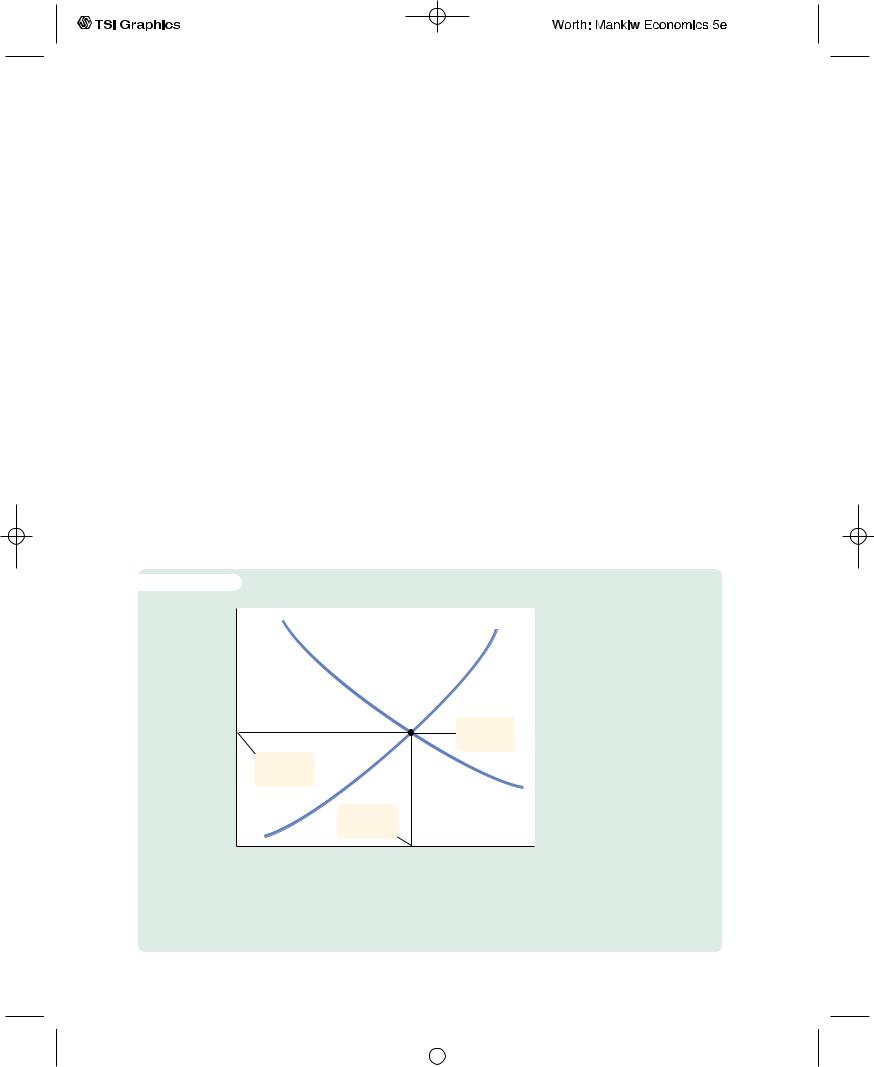
The economist illustrates the model with a supply-and-demand diagram, as in Figure 1-5. The demand curve shows the relationship between the quantity of pizza demanded and the price of pizza, while holding aggregate income constant. The demand curve slopes downward because a higher price of pizza encourages consumers to switch to other foods and buy less pizza.The supply curve shows the relationship between the quantity of pizza supplied and the price of pizza, while holding the price of materials constant.The supply curve slopes upward because a higher price of pizza makes selling pizza more profitable, which encourages pizzerias to produce more of it.The equilibrium for the market is the price and quantity at which the supply and demand curves intersect.At the equilibrium price, consumers choose to buy the amount of pizza that pizzerias choose to produce.

This model of the pizza market has two exogenous variables and two endogenous variables. The exogenous variables are aggregate income and the price of materials.The model does not attempt to explain them but takes them as given (perhaps to be explained by another model). The endogenous variables are the

f i g u r e 1 - 5

Price of pizza, P

Supply

Market equilibrium

Equilibrium price

Demand

Equilibrium quantity

Quantity of pizza, Q

The Model of Supply and Demand

The most famous economic model is that of supply and demand for a good or service—in this case, pizza. The demand curve is a downward-sloping curve relating the price of pizza to the quantity of pizza that consumers demand. The supply curve is an upwardsloping curve relating the price of pizza to the quantity of pizza that pizzerias supply. The price of pizza adjusts until the quantity supplied equals the quantity demanded. The point where the two curves cross is the market equilibrium, which shows the equilibrium price of pizza and the equilibrium quantity of pizza.

User SONPR:Job EFF01417:6264_ch01:Pg 8:24481#/eps at 100% *24481*				Fri, Nov 9, 2001 11:52 AM