01.An introduction to linear control theory

This version: 22/10/2004

Chapter 1

An introduction to linear control theory

With this book we will introduce you to the basics ideas of control theory, and the setting will be that of single-input, single-output (SISO), finite-dimensional, time-invariant, linear systems. In this section we will begin to explore the meaning of this lingo, and look at some simple physical systems which fit into this category. Traditional introductory texts in control may contain some of this material in more detail [see, for example Dorf and Bishop 2001, Franklin, Powell, and Emani-Naeini 1994]. However, our presentation here is intended to be more motivational than technical. For proper background in physics, one should look to suitable references. A very good summary reference for the various methods of deriving equations for physical systems is [Cannon, Jr. 1967].

Contents

1.1	Some control theoretic terminology . . . . . . . . . . . . . . . . . . . . . . . . . . . . . .		1
1.2	An introductory example . . . . . . . . . . . . . . . . . . . . . . . . . . . . . . . . . . . .		2
1.3	Linear di erential equations for physical devices . . . . . . . . . . . . . . . . . . . . . . .		7
	1.3.1	Mechanical gadgets . . . . . . . . . . . . . . . . . . . . . . . . . . . . . . . . . . .	7
	1.3.2	Electrical gadgets . . . . . . . . . . . . . . . . . . . . . . . . . . . . . . . . . . . .	10
	1.3.3	Electro-mechanical gadgets . . . . . . . . . . . . . . . . . . . . . . . . . . . . . . .	11
1.4	Linearisation at equilibrium points . . . . . . . . . . . . . . . . . . . . . . . . . . . . . . .		12
1.5	What you are expected to know . . . . . . . . . . . . . . . . . . . . . . . . . . . . . . . .		13
1.6	Summary . . . . . . . . . . . . . . . . . . . . . . . . . . . . . . . . . . . . . . . . . . . . .		14

1.1 Some control theoretic terminology

For this book, there should be from the outset a picture you have in mind of what you are trying to accomplish. The picture is essentially given in Figure 1.1. The idea is that you are given a plant, which is the basic system, which has an output y(t) that you’d like to do something with. For example, you may wish to track a reference trajectory r(t). One way to do this would be to use an open-loop control design. In this case, one would omit that part of the diagram in Figure 1.1 which is dashed, and use a controller to read the reference signal r(t) and use this to specify an input u(t) to the plant which should give the desired output. This open-loop control design may well work, but it has some inherent problems. If there is a disturbance d(t) which you do not know about, then this may well cause the output of the plant to deviate significantly from the reference

2

1

An introduction to linear control theory

22/10/2004

d(t)

e(t)

u(t)

r(t)

controller

plant

y(t)

−

s(t)

sensor

Figure 1.1 A basic control system schematic

trajectory r(t). Another problem arises with plant uncertainties. One models the plant, typically via di erential equations, but these are always an idealisation of the plant’s actual behaviour. The reason for the problems is that the open-loop control law has no idea what the output is doing, and it marches on as if everything is working according to an idealised model, a model which just might not be realistic. A good way to overcome these di culties is to use feedback. Here the output is read by sensors, which may themselves be modelled by di erential equations, which produce a signal s(t) which is subtracted from the reference trajectory to produce the error e(t). The controller then make its decisions based on the error signal, rather than just blindly considering the reference signal.

1.2 An introductory example

Let’s see how this all plays out in a simple example. Suppose we have a DC servo motor whose output is its angular velocity ω(t), the input is a voltage E(t), and there is a disturbance torque T (t) resulting from, for example, an unknown external load being applied to the output shaft of the motor. This external torque is something we cannot alter. A little later in this section we will see some justification for the governing di erential equations to be given by

dω(t) + 1 ω(t) = kEE(t) + kT T (t). dt τ

The schematic for the situation is shown in Figure 1.2. This schematic representation we

T (t)

kT

u(t)

E(t)

³

d

1

´

ω(t)

kE

+

= u

dt

τ

Figure 1.2

DC motor open-loop control schematic

22/10/2004 1.2 An introductory example 3

give here is one we shall use frequently, and it is called a block diagram.1

Let us just try something na¨ıve and open-loop. The objective is to be able to drive the motor at a specified constant velocity ω0. This constant desired output is then our reference trajectory. You decide to see what you might do by giving the motor some constant torques to see what happens. Let us provide a constant input torque E(t) = E0 and suppose that the disturbance torque T (t) = 0. We then have the di erential equation

ddωt + τ1 ω = kEE0.

Supposing, as is reasonable, that the motor starts with zero initial velocity, i.e., ω(0) = 0, the solution to the initial value problem is

ω(t) = kEE0τ 1 − e−t/τ .

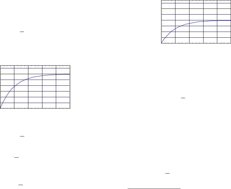
We give a numerical plot for kE = 2, E0 = 3, and τ1 = 12 in Figure 1.3. Well, we say, this all

	14
	12
	10
t)	8
ω(
	6
	4
	2
	2	4	6	8	10
			t

Figure 1.3 Open-loop response of DC motor

looks too easy. To get the desired output velocity ω0 after a su ciently long time, we need

only provide the input voltage E0 = ω0 .

τkE

However, there are decidedly problems lurking beneath the surface. For example, what if there is a disturbance torque? Let us suppose this to be constant for the moment so T (t) = −T0 for some T0 > 0. The di erential equation is then

ddωt + τ1 ω = kEE0 − kT T0,

and if we again suppose that ω(0) = 0 the initial value problem has solution

ω(t) = (kEE0 − kT T0)τ 1 − e−t/τ .

If we follow our simple rule of letting the input voltage E0 be determined by the desired final

angular velocity by our rule E0 = ω0 , then we will undershoot our desired final velocity

kEτ

by ωerror = kT T0τ. In this event, the larger is the disturbance torque, the worse we do—in

4

1 An introduction to linear control theory

22/10/2004

	14
	12
	10
t)	8
ω(
	6
	4
	2
	2	4	6	8	10
			t

Figure 1.4 Open-loop response of DC motor with disturbance

fact, we can do pretty darn bad if the disturbance torque is large. The e ect is illustrated in Figure 1.4 with kT = 1 and T0 = 2.

Another problem arises when we have imperfect knowledge of the motor’s physical characteristics. For example, we may not know the time-constant τ as accurately as we’d like. While we estimate it to be τ, it might be some other value τ˜. In this case, the actual di erential equation governing behaviour in the absence of disturbances will be

ddωt + τ1˜ ω = kEE0, which gives the solution to the initial value problem as

ω(t) = kEE0τ˜ 1 − e−t/τ˜ .

The final value will then be in error by the factor ττ˜ . This situation is shown in Figure 1.5

for τ1˜ = 58 .

Okay, I hope now that you can see the problem with our open-loop control strategy. It simply does not account for the inevitable imperfections we will have in our knowledge of the system and of the environment in which it works. To take all this into account, let us measure the output velocity of the motor’s shaft with a tachometer. The tachometer takes the angular velocity and returns a voltage. This voltage, after being appropriately scaled by a factor ks, is then compared to the voltage needed to generate the desired velocity by feeding it back to our reference signal by subtracting it to get the error. The error we multiply by some constant K, called the gain for the controller, to get the actual voltage input to the system. The schematic now becomes that depicted in Figure 1.6. The di erential equations governing this system are

ddωt + (τ1 + kEkSK)ω = kEKωref + kT T.

We shall see how to systematically obtain equations such as this, so do not worry if you think it in nontrivial to get these equations. Note that the input to the system is, in some

1When we come to use block diagrams for real, you will see that the thing in the blocks are not di erential equations in the time-domain, but in the Laplace transform domain.

22/10/2004

1.2 An introductory example

5

	14
	12
	10
t)	8
ω(
	6
	4
	2
	2	4	6	8	10
			t

Figure 1.5 Open-loop response of DC motor with “actual” motor time-constant

T (t)

plant

controller

kT

u(t)

ωref

E

³

d

1

´

ω(t)

K

kE

+

= u

−

dt

τ

sensor

kS

Figure 1.6 DC motor closed-loop control schematic

sense, no longer the voltage, but the reference signal ωref. Let us suppose again a constant disturbance torque T (t) = −T0 and a constant reference voltage ωref = ω0. The solution to the di erential equation, again supposing ω(0) = 0, is then

ω(t) = kEKω0 − kT T0 1 − e−( τ1 +kEkSK)t .

τ1 + kEkSK

Let us now investigate this closed-loop control law. As previously, let us first look at the case when T0 = 0 and where we suppose perfect knowledge of our physical constants and our model. In this case, we wish to achieve a final velocity of ω0 = E0τkE as t → ∞, i.e., the same velocity as we had attained with our open-loop strategy. We see the results of this in Figure 1.7 where we have chosen kS = 1 and K = 5. Notice that the motor no longer achieves the desired final speed! However, we have improved the response time for the system

6

1 An introduction to linear control theory

22/10/2004

	14
	12
	10
t)	8
ω(
	6
	4
	2
	2	4	6	8	10
			t

Figure 1.7 Closed-loop response of DC motor

significantly from the open-loop controller (cf. Figure 1.3). It is possible to remove the final error by doing something more sophisticated with the error than multiplying it by K, but we will get to that only as the course progresses. Now let’s see what happens when we add a constant disturbance by setting T0 = 2. The result is displayed in Figure 1.8. We

	14
	12
	10
t)	8
ω(
	6
	4
	2
	2	4	6	8	10
			t

Figure 1.8 Closed-loop response of DC motor with disturbance

see that the closed-loop controller reacts much better to the disturbance (cf. Figure 1.4), although we still (unsurprisingly) cannot reach the desired final velocity. Finally we look at the situation when we have imperfect knowledge of the physical constants for the plant. We again consider having τ1˜ = 58 rather than the guessed value of 12 . In this case the closed-loop response is shown in Figure 1.9. Again, the performance is somewhat better than that of the open-loop controller (cf. Figure 1.5), although we have incurred a largish final error in the final velocity.

I hope this helps to convince you that feedback is a good thing! As mentioned above, we shall see that it is possible to design a controller so that the steady-state error is zero, as this is the major deficiency of our very basic controller “designed” above. This simple example, however, does demonstrate that one can achieve improvements in some areas (response time

22/10/2004

1.3 Linear di erential equations for physical devices

7

	14
	12
	10
t)	8
ω(
	6
	4
	2
	2	4	6	8	10
			t

Figure 1.9 Closed-loop response of DC motor with “actual” motor time-constant

in this case), although sometimes at the expense of deterioration in others (steady-state error in this case).

1.3 Linear di erential equations for physical devices

We will be considering control systems where the plant, the controller, and the sensors are all modelled by linear di erential equations. For this reason it makes sense to provide some examples of devices whose behaviour is reasonably well-governed by such equations. The problem of how to assemble such devices to, say, build a controller for a given plant is something we will not be giving terribly much consideration to.

1.3.1 Mechanical gadgets In Figure 1.10 is a really feeble idealisation of a car suspension system. We suppose that at y = 0 the mass m is in equilibrium. The spring, as we

F (t)

y(t)

m

k d

Figure 1.10 Simplified automobile suspension

know, then supplies a restoring force Fk = −ky and the dashpot supplies a force Fd = −dy˙, where “ ˙ ” means ddt . We also suppose there to be an externally applied force F (t). If we ask Isaac Newton, “Isaac, what are the equations governing the behaviour of this system?”

8 1 An introduction to linear control theory 22/10/2004

he would reply, “Well, F = ma, now go think on it.”2 After doing so you’d arrive at my¨(t) = F (t) − ky(t) − dy˙(t) = my¨(t) + dy˙(t) + ky(t) = F (t).

This is a second-order linear di erential equation with constant coe cients and with inhomogeneous term F (t).

The same sort of thing happens with rotary devices. In Figure 1.11 is a rotor fixed to a shaft moving with angular velocity ω. Viscous dissipation may be modelled with a force

ω(t)

Figure 1.11 Rotor on a shaft

proportional to the angular velocity: Fd = −dω. In the presence of an external torque τ(t), the governing di erential equation is

Jω˙ (t) + dω(t) = τ(t)

where J is the moment of inertia of the rotor about its point of rotation. If one wishes to include a rotary spring, then one must consider not the angular velocity ω(t) as the dependent variable, but rather the angular displacement θ(t) = θ0 + ωt. In either case, the governing equations are linear di erential equations.

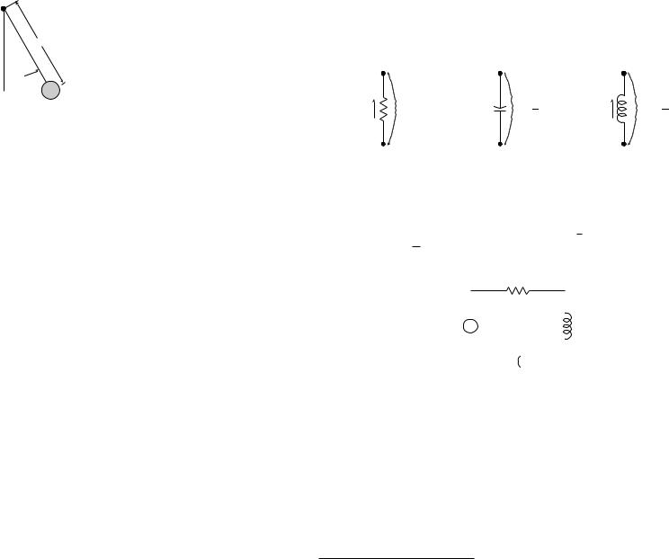
Let’s look at a simple pendulum (see Figure 1.12). If we sum moments about the pivot we get

2 ¨	=	¨	g	sin θ = 0.
m` θ = −mg` sin θ		θ +	`

Now this equation, you will notice, is nonlinear. However, we are often interested in the behaviour of the system near the equilibrium points which are (θ, θ˙) = (θ0, 0) where θ0 {0, π}. So, let us linearise the equations near these points, and see what we get. We write the solution near the equilibrium as θ(t) = θ0 + ξ(t) where ξ(t) is small. We then have

¨

g

¨

g

¨

g

g

θ +

` sin θ = ξ +

` sin(θ0

+ ξ) = ξ +

` sin θ0 cos ξ + ` cos θ0 sin ξ.

−

0

0

{

}

0

0

x3

x5

Now note that sin θ

= 0 if θ

0, π

, and cos θ

= 1 if θ

= 0 and cos θ0

=

1 if θ0

= π.

We also use the Taylor expansion for sin x around x = 0: sin x = x −

+

+ . . . . Keeping

3!

5!

2This is in reference to the story, be it true or false, that when Newton was asked how he’d arrived at the inverse square law for gravity, he replied, “I thought on it.”

22/10/2004

1.3 Linear di erential equations for physical devices

9

`

θ

Figure 1.12 A simple pendulum

only the lowest order terms gives the following equations which should approximate the behaviour of the system near the equilibrium (θ0, 0):

¨	g	ξ = 0, θ0	= 0
ξ +	`
¨	g		= π.
ξ −	` ξ = 0, θ0

In each case, we have a linear di erential equation which governs the behaviour near the equilibrium. This technique of linearisation is ubiquitous since there really are no linear physical devices, but linear approximations seem to work well, and often very well, particularly in control. We discuss linearisation properly in Section 1.4.

Let us recall the basic rules for deriving the equations of motion for a mechanical system.

1.1 Deriving equations for mechanical systems Given: an interconnection of point masses and rigid bodies.

1.Define a reference frame from which to measure distances.

2.Choose a set of coordinates that determine the configuration of the system.

3.Separate the system into its mechanical components. Thus each component should be either a single point mass or a single rigid body.

4.For each component determine all external forces and moments acting on it.

5.For each component, express the position of the centre of mass in terms of the chosen coordinates.

6.The sum of forces in any direction on a component should equal the mass of the component times the component of acceleration of the component along the direction of the force.

7.For each component, the sum of moments about a point that is either (a) the centre of mass of the component or (b) a point in the component that is stationary should equal

the moment of inertia of the component about that point multiplied by the angular acceleration.

This methodology has been applied to the examples above, although they are too simple to be really representative. We refer to the exercises for examples that are somewhat more interesting. Also, see [Cannon, Jr. 1967] for details on the method we outline, and other methods.

10

1 An introduction to linear control theory

22/10/2004

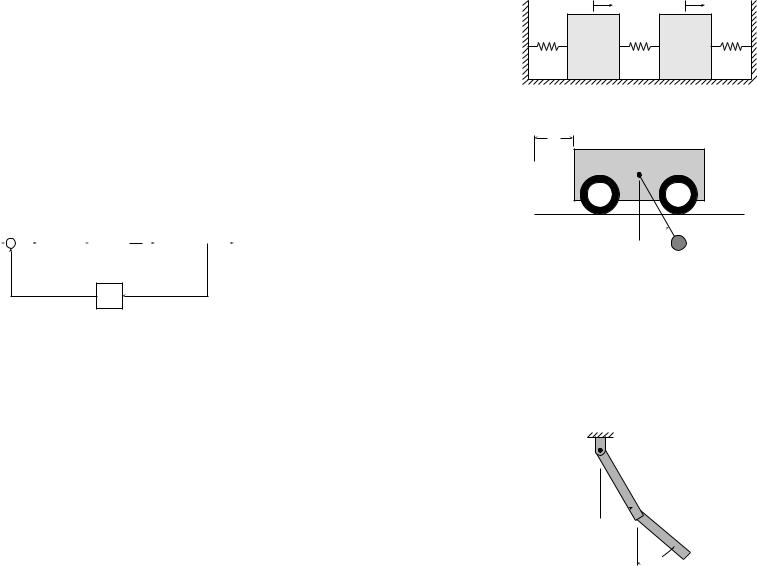
1.3.2 Electrical gadgets A resistor is a device across which the voltage drop is proportional to the current through the device. A capacitor is a device across which the voltage drop is proportional to the charge in the device. An inductor is a device across which the voltage drop is proportional to the time rate of change of current through the device. The three devices are typically given the symbols as in Figure 1.13. The quantity

I (t)	E = RI	q(t)	E = C1 q	I (t)	E = L ddIt
Resistor		Capacitor			Inductor

Figure 1.13 Electrical devices

R is called the resistance of the resistor, the quantity C is called the capacitance of the capacitor, and the quantity L is called the inductance of the inductor. Note that the proportionality constant for the capacitor is not C but C1 . The current I is related to the charge q by I = ddqt . We can then imagine assembling these electrical components in some configuration and using Kirchho ’s laws3 to derive governing di erential equations. In Figure 1.14 we have a particularly simple configuration. The voltage drop around the circuit

		R
	+
E				L
	−	C

Figure 1.14			A series RLC circuit
must be zero which gives the governing equations
E(t) = RI(t) + LI˙(t) +	1	q(t)	= Lq¨(t) + Rq˙(t) +	1	q(t) = E(t)
	C			C

where E(t) is an external voltage source. This may also be written as a current equation by merely di erentiating:

¨	˙	1	˙
LI(t) + RI(t) +		C	I(t) = E(t).

In either case, we have a linear equation, and again one with constant coe cients.

Let us present a methodology for determining the di erential equations for electric circuits. The methodology relies on the notion of a tree which is a connected collection of branches containing no loops. For a given tree, a tree branch is a branch in the tree, and a link is a branch not in the tree.

3Kirchho ’s voltage law states that the sum of voltage drops around a closed loop must be zero and Kirchho ’s current law states that the sum of the currents entering a node must be zero.

22/10/2004 1.3 Linear di erential equations for physical devices 11

1.2 Deriving equations for electric circuits Given: an interconnection of ideal resistors, capacitors, and inductors, along with voltage and current sources.

1.Define a tree by collecting together a maximal number of branches to form a tree. Add elements in the following order of preference: voltage sources, capacitors, resistors, inductors, and current sources. That is to say, one adds these elements in sequence until one gets the largest possible tree.

2.The states of the system are taken to be the voltages across capacitors in the tree branches for the tree of part 1 and the currents through inductors in the links for the tree from part 1.

3.Use Kirchho ’s Laws to derive equations for the voltage and current in every tree branch in terms of the state variables.

4.Write the Kirchho Voltage Law and the Kirchho Current Law for every loop and every

node corresponding to a branch assigned a state variable.

The exercises contain a few examples that can be used to test one’s understanding of the above method. We also refer to [Cannon, Jr. 1967] for further discussion of the equations governing electrical networks.

1.3.3 Electro-mechanical gadgets If you really want to learn how electric motors work, then read a book on the subject. For example, see [Cannon, Jr. 1967].

A DC servo motor works by running current through a rotary toroidal coil which sits in a stationary magnetic field. As current is run through the coil, the induced magnetic field induces the rotor to turn. The torque developed is proportional to the current through the coil: T = KtI where T is the torque supplied to the shaft, I is the current through the coil, and Kt is the “torque constant.” The voltage drop across the motor is proportional to the motor’s velocity; Em = Keθ˙ where Em is the voltage drop across the motor, Ke is a constant, and θ is the angular position of the shaft. If one is using a set of consistent units with velocity measured in rads/sec, then apparently Ke = Kt.

Now we suppose that the rotor has inertia J and that shaft friction is viscous and so the friction force is given by −dθ˙. Thus the motor will be governed by Newton’s equations:

¨	˙	=	¨ ˙
Jθ = −dθ + KtI			Jθ + dθ = KtI.

To complete the equations, one need to know the relationship between current and θ. This is provided by the relation Em = Keθ˙ and the dynamics of the circuit which supplies current to the motor. For example, if the circuit has resistance R and inductance L then we have

LddIt + RI = E − Keθ˙

with E being the voltage supplied to the circuit. This gives us coupled equations

¨

˙

Jθ + dθ = KtI

L

dI

+ RI = E − Keθ˙

dt

which we can write in first-order system form as

1

−K

R

θ˙

0

1

0

θ

0

v˙θ

=

0

d

Kt

vθ

+

0

E

J

J

I˙

0

−

e

−L

I

L

L

12

1 An introduction to linear control theory

22/10/2004

where we define the dependent variable vθ = θ˙. If the response of the circuit is much faster than that of the motor, e.g., if the inductance is small, then this gives E = Keθ˙ + RI and so the equations reduce to

Jθ¨ +	d + KtR e θ˙ =		Rt E.
		K	K

Thus the dynamics of a DC motor can be roughly described by a first-order linear di erential equation in the angular velocity. This is what we saw in our introductory example.

Hopefully this gives you a feeling that there are a large number of physical systems which are modelled by linear di erential equations, and it is these to which we will be restricting our attention.

1.4 Linearisation at equilibrium points

When we derived the equations of motion for the pendulum, the equations we obtained were nonlinear. We then decided that if we were only interested in looking at what is going on near an equilibrium point, then we could content ourselves with linearising the equations. We then did this in a sort of hacky way. Let’s see how to do this methodically.

We suppose that we have vector di erential equations of the form

x˙1 = f1(x1, . . . , xn) x˙2 = f2(x1, . . . , xn)

.

.

.

x˙n = fn(x1, . . . , xn).

The n functions (f1, . . . , fn) of the n variables (x1, . . . , xn) are known smooth functions. Let us denote x = (x1, . . . , xn) and f(x) = (f1(x), . . . , fn(x)). The di erential equation can then be written as

x˙ = f(x).

(1.1)

It really only makes sense to linearise about an equilibrium point. An equilibrium point is a point x0 Rn for which f(x0) = 0. Note that the constant function x(t) = x0 is a solution to the di erential equation if x0 is an equilibrium point. For an equilibrium point x0 define an n × n matrix Df(x0) by

∂f1

(x0)

∂f1

(x0) · · ·

∂f1

(x0)

∂x1

∂x2

∂xn

∂x1

(x0)

∂x2

(x0)

· · ·

∂xn

(x0)

∂f2

∂f2

..

...

∂f2

..

..

Df(x0) =

.

.

.

)

.

∂fn

(x

)

∂fn

(x

)

∂fn

(x

∂x1

∂x2

∂xn

0

0

· · ·

0

This matrix is often called the Jacobian of f at x0. The linearisation of (1.1) about an equilibrium point x0 is then the linear di erential equation

ξ˙ = Df(x0)ξ.

Let’s see how this goes with our pendulum example.

1.3Example The nonlinear di erential equation we derived was

¨g

θ+ ` sin θ = 0.

22/10/2004

1.5 What you are expected to know

13

This is not in the form of (1.1) since it is a second-order equation. But we can put this into first-order form by introducing the variables x1 = θ and x2 = θ˙. The equations can then be written

x˙1 = θ˙ = x2

x˙	¨	−	g	sin θ = −	g	sin x1.
	2 = θ =		`		`
Thus							g
				f2(x1, x2) = −
f1(x1, x2) = x2		,						sin x1.
							`

Note that at an equilibrium point we must have x2 = 0. This makes sense as it means that the pendulum should not be moving. We must also have sin x1 = 0 which means that x1 {0, π}. This is what we determined previously.

Now let us linearise about each of these equilibrium points. For an arbitrary point x = (x1, x2) we compute

0		1
Df(x) = −g` cos x1		0 .
At the equilibrium point x1 = (0, 0) we thus have	0
Df(x1) = −g`		,
0	1
and at the equilibrium point x2 = (0, π) we thus have
Df(x1) = g`	0 .
0	1

With these matrices at hand, we may write the linearised equations at each equilibrium point.

1.5 What you are expected to know

There are five essential areas of background that are assumed of a student using this text. These are

1.linear algebra,

2.ordinary di erential equations, including the matrix exponential,

3.basic facts about polynomials,

4.basic complex analysis, and

5.transform theory, especially Fourier and Laplace transforms.

Appendices review each of these in a cursory manner. Students are expected to have seen this material in detail in previous courses, so there should be no need for anything but rapid review in class.

Many of the systems we will look at in the exercises require in their analysis straightforward, but tedious, calculations. It should not be the point of the book to make you go through such tedious calculations. You will be well served by learning to use a computer package for doing such routine calculations, although you should try to make sure you are asking the computer to do something which you in principle understand how to do yourself.

14

1 An introduction to linear control theory

22/10/2004

I have used Mathematica® to do all the plotting in the book since it is what I am familiar with. Also available are Maple® and Matlab®. Matlab® has a control toolbox, and is the most commonly used tool for control systems.4

You are encouraged to use symbolic manipulation packages for doing problems in this book. Just make sure you let us know that you are doing so, and make sure you know what you are doing and that you are not going too far into black box mode.

1.6 Summary

Our objective in this chapter has been to introduce you to some basic control theoretic ideas, especially through the use of feedback in the DC motor example. In the remainder of these notes we look at linear systems, and to motivate such an investigation we presented some physical devices whose behaviour is representable by linear di erential equations, perhaps after linearisation about a desired operating point. We wrapped up the chapter with a quick summary of the background required to proceed with reading these notes. Make sure you are familiar with everything discussed here.

4Mathematica® and Maple® packages have been made available on the world wide web for doing things such as are done in this book. See http://mast.queensu.ca/~math332/.

Exercises for Chapter 1

15

Exercises

E1.1 Probe your life for occurrences of things which can be described, perhaps roughly, by a schematic like that of Figure 1.1. Identify the components in your system which are the plant, output, input, sensor, controller, etc. Does your system have feedback? Are there disturbances?

E1.2 Consider the DC servo motor example which we worked with in Section 1.2. Determine conditions on the controller gain K so that the voltage E0 required to obtain a desired steady-state velocity is greater for the closed-loop system than it is for the openloop system. You may neglect the disturbance torque, and assume that the motor model is accurate. However, do not use the numerical values used in the notes—leave everything general.

E1.3 An amplifier is to be designed with an overall amplification factor of 2500 ± 50. A number of single amplifier stages is available and the gain of any single stage may drift anywhere between 25 and 75. The configuration of the final amplifier is given in Figure E1.1. In each of the blocks we get to insert an amplifier stage with the large

Vin

K1

K2

KN

Vout

−

α

Figure E1.1 A multistage feedback amplifier

and unknown gain variation (in this case the gain variation is at most 50). Thus the gain in the forward path is K1K2 · · · KN where N is the number of amplifier stages and where Ki [25, 75]. The element in the feedback path is a constant 0 < α < 1.

(a) For N amplifier stages and a given value for α determine the relationship between

Vin and Vout.

The feedback gain α is known precisely since it is much easier to design a circuit which provides accurate voltage division (as opposed to amplification). Thus, we can assume that α can be exactly specified by the designer.

(b)Based on this information find a value of α in the interval (0, 1) and, for that value of α, the minimal required number of amplifier stages, Nmin, so that the final amplifier design meets the specification noted above.

E1.4 Derive the di erential equations governing the behaviour of the coupled masses in Figure E1.2. How do the equations change if viscous dissipation is added between each mass and the ground? (Suppose that both masses are subject to the same dissipative force.)

The following two exercises will recur as exercises in succeeding chapters. Since the computations can be a bit involved—certainly they ought to be done with a symbolic manipulation package—it is advisable to do the computations in an organised manner so that they may be used for future calculations.

16

1 An introduction to linear control theory

22/10/2004

	x1	x2
k	k	k
	m	m

Figure E1.2 Coupled masses

x

θ

Figure E1.3 Pendulum on a cart

E1.5 Consider the pendulum on a cart pictured in Figure E1.3. Derive the full equations which govern the motion of the system using coordinates (x, θ) as in the figure. Here M is the mass of the cart and m is the mass of the pendulum. The length of the pendulum arm is `. You may assume that there is no friction in the system. Linearise the equations about the points (x, θ, x,˙ θ˙) = (x0, 0, 0, 0) and (x, θ, x,˙ θ˙) = (x0, π, 0, 0), where x0 is arbitrary.

E1.6 Determine the full equations of motion for the double pendulum depicted in Figure E1.4. The first link (i.e., the one connected to ground) has length `1 and mass

θ1

θ2

Figure E1.4 Double pendulum

m1, and the second link has length `2 and mass m2. The links have a uniform mass density, so their centres of mass are located at their midpoint. You may assume that

Exercises for Chapter 1

17

there is no friction in the system. What are the equilibrium points for the double pendulum (there are four)? Linearise the equations about each of the equilibria.

E1.7 Consider the electric circuit of Figure E1.5. To write equations for this system we

	R
	+
E	C	L
	−

Figure E1.5 Electric circuit

need to select two system variables. Using IC, the current through the capacitor, and IL, the current through the inductor, derive a first-order system of equations in two variables governing the behaviour of the system.

E1.8 For the circuit of Figure E1.6, determine a di erential equation for the current through

	R1
	+
E	R2	C

−

Figure E1.6 Another electric circuit

the resistor R1 in terms of the voltage E(t).

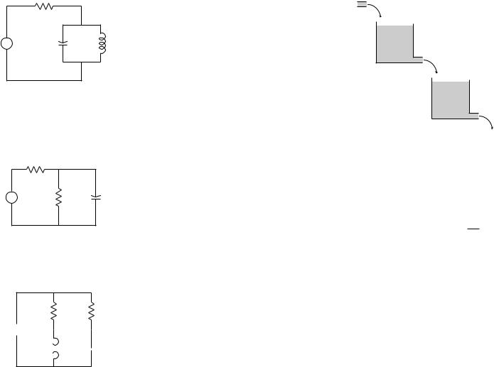
E1.9 For the circuit of Figure E1.7, As dependent variable for the circuit, use the volt-

RL RC

+

E

−

L C

Figure E1.7 Yet another electric circuit

age across the capacitor and the current through the inductor. Derive di erential equations for the system as a first-order system with two variables.

18

1 An introduction to linear control theory

22/10/2004

E1.10 The mass flow rate from a tank of water with a uniform cross-section can be roughly modelled as being proportional to the height of water in the tank which lies above the exit nozzle. Suppose that two tanks are configured as in Figure E1.8 (the tanks

Figure E1.8 Coupled water tanks

are not necessarily identical). Determine the equations of motion which give the mass flow rate from the bottom tank given the mass flow rate into the top tank. In this problem, you must define the necessary variables yourself.

In the next exercise we will consider a more complex and realistic model of flow in coupled tanks. Here we will use the Bernoulli equation for flow from small orifices. This says that if a tank of uniform cross-section has fluid level h, then√the velocity flowing from a small nozzle at the bottom of the tank will be given by v = 2gh, where g is the gravitational acceleration.

E1.11 Consider the coupled tanks shown in Figure E1.9. In this scenario, the input is the volume flow rate Fin which gets divided between the two tanks proportionally to the

areas α1 and α2 of the two tubes. Let us denote α =	α1	.
	α1+α2

(a)Give an expression for the volume flow rates Fin,1 and Fin,2 in terms of Fin and α.

Now suppose that the areas of the output nozzles for the tanks are a1 and a2, and that the cross-sectional areas of the tanks are A1 and A2. Denote the water levels in the tanks by h1 and h2.

(b)Using the Bernoulli equation above, give an expression for the volume flow rates Fout,1 and Fout,2 in terms of a1, a2, h1, and h2.

(c)Using mass balance (assume that the fluid is incompressible so that mass and volume balance are equivalent), provide two coupled di erential equations for the heights h1 and h2 in the tanks. The equations should be in terms of Fin, α, A1, A2, a1, a2, and g, as well as the dependent variables h1 and h2.

Suppose that the system is in equilibrium (i.e., the heights in the tanks are constant) with the equilibrium height in tank 1 being δ1.

(d)What is the equilibrium input flow rate ν?

(e)What is the height δ2 of fluid in tank 2?

Exercises for Chapter 1

19

20

1 An introduction to linear control theory

22/10/2004

Fin
α1	α2
Fin,1
A1
a1
	Fout,1
	Fin,2
	A2
	a2

Fout,2

Figure E1.9 Another coupled tank scenario