02.System modelling

change immediately when the gas pedal is pushed nor does the temperature in a room rise instantaneously when an air conditioner is switched on. Similarly, a headache does not vanish right after an aspirin is taken, requiring time to take e®ect. In business systems, increased funding for a development project does not increase revenues in the short term, although it may do so in the long term (if it was a good investment). All of these are examples of dynamical systems, in which the behavior of the system evolves with time.

Dynamical systems can be viewed in two di®erent ways: the internal view or the external view. The internal view attempts to describe the internal workings of the system and originates from classical mechanics. The prototype problem was describing the motion of the planets. For this problem it was natural to give a complete characterization of the motion of all planets. This involves careful analysis of the e®ects of gravitational pull and the relative positions of the planets in a system.

The other view on dynamics originated in electrical engineering. The prototype problem was to describe electronic ampli¯ers. It was natural to view an ampli¯er as a device that transforms input voltages to output voltages and disregard the internal detail of the ampli¯er. This resulted in the input/output view of systems. The two di®erent views have been amalgamated in control theory. Models based on the internal view are called internal descriptions, state models, or white box models. The external view is associated with names such as external descriptions, input/output models or black box models. In this book we will mostly use the words state models and input/output models.

In the remainder of this section we provide an overview of some of the key concepts in modeling. The mathematical details introduced here are explored more fully in the remainder of the chapter.

The Heritage of Mechanics

The study of dynamics originated in the attempts to describe planetary motion. The basis was detailed observations of the planets by Tycho Brahe and the results of Kepler who found empirically that the orbits of the planets could be well described by ellipses. Newton embarked on an ambitious program to try to explain why the planets move in ellipses and he found that the motion could be explained by his law of gravitation and the formula that force equals mass times acceleration. In the process he also invented calculus and di®erential equations. Newton's result was the ¯rst example of the idea of reductionism, i.e. that seemingly complicated natural phenomena can be explained by simple physical laws. This became the paradigm of natural

science for many centuries.

One of the triumphs of Newton's mechanics was the observation that the motion of the planets could be predicted based on the current positions and velocities of all planets. It was not necessary to know the past motion. The state of a dynamical system is a collection of variables that characterize the motion of a system completely for the purpose of predicting future motion. For a system of planets the state is simply the positions and the velocities of the planets. We call the set of all possible states the state space.

A common class of mathematical models for dynamical systems is ordinary di®erential equations (ODEs). Mathematically, an ODE is written as

Here x = (x1; x2; : : : ; xn) 2 Rn is a vector of real numbers that describes the current state of the system and equation (2.1) describes the rate of change of the state as a function of the state itself. Note that we do not bother to write the vector x any di®erently than a scalar variable. It will generally be clear from context whether a variable is a vector or scalar quantity.

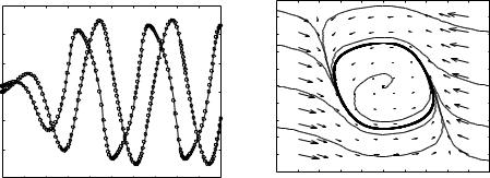
An example of an ordinary di®erential equation is the van der Pol equation,

dx1 3

dt = x1 ¡ x1 ¡ x2 (2.2) dx2

dt

which is a model of an electronic oscillator. The state of the system is represented by two real numbers, x1 and x2. The model (2.2) gives the velocity of the state vector for each value of the state.

The evolution of the states can be described using either a time plot or a phase plot, both of which are shown in Figure 2.1. The time plot, on the left, shows the values of the individual states as a function of time. The phase plot, on the right, shows the vector ¯eld for the system, which gives the state velocity (represented as an arrow) at every point in the state space. In addition, we have superimposed the traces of some of the states from di®erent conditions. The phase plot gives a strong intuitive representation of the equation as a vector ¯eld or a °ow. While systems of second order (two states) can be represented in this way, it is unfortunately di±cult to visualize equations of higher order using this approach.

The ideas of dynamics and state have had a profound in°uence on philosophy where they inspired the idea of predestination. If the state of a natural system is known at some time, its future development is completely

Vout

Vin

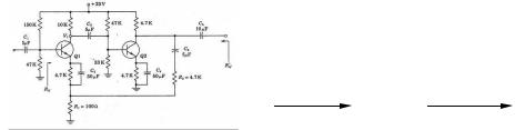
Figure 2.2: Illustration of the input/output view of a dynamical system. The ¯gure on the left shows a detailed circuit diagram for an electronic ampli¯er; the one of the right its representation as a block diagram.

we can examine what in°uence external disturbances have on the trajectories of a system. Or, in the case when the input variable is something that can be modulated in a controlled way, we can analyze whether it is possible to \steer" the system from one point in the state space to another through proper choice of the input.

The Heritage of Electrical Engineering

A very di®erent view of dynamics emerged from electrical engineering, where the design of electronic ampli¯ers led to a focus on input/output behavior. A system was considered as a device that transformed inputs to outputs, as illustrated in Figure 2.2. Conceptually an input/output model can be viewed as a giant table of inputs and outputs.

The input/output framework is used in many engineering systems since it allows us to decompose a problem into individual components, connected through their inputs and outputs. Thus, we can take a complicated system such as a radio or a television and break it down into manageable pieces, such as the receiver, demodulator, ampli¯er, and speakers. Each of these pieces has a set of inputs and outputs and, through proper design, these components can be interconnected to form the entire system.

The input/output view is particularly useful for the special class of linear, time-invariant systems. To de¯ne linearity, we let (u1; y1) and (u2; y2) denote two input/output pairs|i.e., the input u1 produces the (unique) output y1|and a and b be real numbers. A system is linear if (au1 + bu2; ay1 + by2) is also an input/output pair; this is often called the principle of superposition. A system is time-invariant if the output response for a

given input does not depend on when that input is applied. More formally, we let u¿ denote a signal obtained by shifting the signal u by ¿ units of time. If (u; y) is an input/output pair, then the system is called time-invariant if (ut; yt) is also an input output pair. Thus, applying an input now or t seconds from now will generate the same output, just shifted in time. (Chapter 4 provides a much more detailed analysis of linear systems.)

Many electrical engineering systems can be modeled by linear, timeinvariant systems and hence a large number of tools have been developed to analyze them. For example, the step response of a linear system describes the relationship between an input that changes from zero to a constant value abruptly (a \step" input) and the corresponding output. As we shall see in the latter part of the text, the step response is extremely useful in characterizing the performance of a dynamical system and it is often used to specify the desired dynamics.

Another possibility to describe a linear, time-invariant system is to represent the system by its response to sinusoidal input signals. This is called the frequency response and a rich powerful theory with many concepts and strong, useful results have emerged. The results are based on the theory of complex variables and Laplace transforms.

The input/output view lends it naturally to experimental determination of system dynamics, where a system is characterized by recording its response to a particular input, e.g. a step.

The Control View

When control emerged in the 1940s, the approach to dynamics was strongly in°uenced by the electrical engineering view. The second wave of developments, starting in the late 1950s, was inspired by mechanics and the two di®erent views were merged. Systems like planets are autonomous and cannot easily be in°uenced from the outside. Much of the classical development of dynamical systems therefore focused on autonomous systems. In control it is of course essential that systems can have external in°uences. The emergence of space °ight is a typical example where precise control of the orbit is essential. Information also plays an important role in control because it is essential to know the information about a system that is provided by available sensors.

The models from mechanics were thus modi¯ed to include external control forces and sensors. In control, the model given by equation (2.1) was

y = g(x; u);

where u is a vector of control signal and y a vector of measurements. This viewpoint has added to the richness of the classical problems and led to new concepts. For example it is natural to ask if possible states x state space can be reached with the proper choice of u (reachability) and if the measurement contains enough information to reconstruct the state (observability).

The input/output approach was also strengthened by using ideas from functional analysis to deal with nonlinear systems. Relations between the state view and the input output view were also established. Current control theory presents a rich view of dynamics based on good classical traditions.

The importance of disturbances and model uncertainty are critical elements of control because these are the main reasons for using feedback. To model disturbances and model uncertainty is therefore essential. One approach is to describe a model by a nominal system and some characterization of the model uncertainty. The dual views on dynamics is essential in this context. State models are very convenient to describe a nominal model but uncertainties are easier to describe using input/output models (often via a frequency response description).

Modeling from Experiments

Since control systems are provided with sensors and actuators it is also possible to obtain models of system dynamics from experiments on the process. The models are restricted to input/output models since only these signals are accessible to experiments, but modeling from experiments can also be combined with modeling from physics through the use of feedback and interconnection.

The static relation between inputs and outputs can easily be established by determining the steady state response to constant input signals. If the system is unstable or if it has a slow response time the experiment can be performed in closed loop with a simple controller connected to the process. An experiment of this type tells directly if the process is nonlinear.

A simple way to determine dynamics is to observe the response to a step change in the control signal. Such an experiment begins by setting the control signal to a constant value, then steady state is established the control signal is changed quickly to a new level and the output is observed. The experiment will thus directly give the step response of the system. The shape

of the response gives useful information about the dynamics. It immediately gives an indication of the response time and it tells if the system is oscillatory or if the response in monotone. By repeating the experiment for di®erent steady state values and di®erent amplitudes of the change of the control signal we can also determine ranges where the process can be approximated by a linear system.

Modeling from experiments can also be done using many other signals. Sinusoidal signals are commonly used particularly for systems with fast dynamics. Very precise measurements can be obtained by exploiting correlation techniques. An indication of nonlinearities can be obtained by repeating experiments with input signals having di®erent amplitudes.

2.2State Space Models

In this section we introduce the two primary forms of models that we use in this text: di®erential equations and di®erence equations. Both of these make use of the notions of state, inputs, outputs and dynamics to describe the behavior of a system.

Ordinary Di®erential Equations

The state is a collection of variables that summarize the past of a system for the purpose of prediction the future. For an engineering system the state is composed of the variables required to account for storage of mass, momentum and energy. A key issue in modeling is to decide how accurately this storage has to be represented. The state variables are gathered in a vector, x 2 Rn, called the state vector. The control variables are represented by another vector u 2 Rp and the measured signal by the vector y 2 Rq . A system can then be represented by the di®erential equation

x = f (x; u)

(2.5)

y = g(x; u);

where x = dx=dt. We call a model of this form a state space model.

The dimension of the state vector is called the order of the system. The system is called time-invariant because the functions f and g do not depend explicitly on time t. It is possible to have more general time-varying systems where the functions do depend on time. The model thus consists of two functions. The function f gives the velocity of the state vector as

a function of state x and control u, and the function g gives the measured values as functions of state x and control u.

A system is called linear if the functions f and g are linear in x and u. A linear state space system can thus be represented by

x = Ax + Bu

y = Cx + Du;

where A, B, C and D are constant matrices. Such a system is said to be linear and time-invariant, or LTI for short. The matrix A is called the dynamics matrix, the matrix B is called the control matrix, the matrix C is called the sensor matrix and the matrix D is called the direct term. Frequently systems will not have a direct term, indicating that the control signal does not in°uence the output directly.

A di®erent form of linear di®erential equations, perhaps more familiar to many readers, is an equation of the form

where t is the independent (time) variable, y(t) is the dependent (output) variable, and u(t) is the input. This system can be converted into state space form by de¯ning

and the state space equations become

y = x1:

With the appropriate de¯nition of A, B, C and D, this equation is in linear state space form.

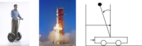
Figure 2.3: Balance systems: (a) Segway human transportation systems,

(b) Saturn rocket and (c) simpli¯ed diagram. Each of these examples uses forces at the bottom of the system to keep it upright.

A more general system is obtained by letting the output be a linear combination of the states of the system, i.e.

y = bnx1 + bn¡1x2 + ¢¢¢ + b1xn + du

This system can be modeled in state space as

Example 2.1 (Balance systems). An example of a class of systems that can be modeled using ordinary di®erential equations is the class of \balance systems." A balance system is a mechanical system in which the center of mass is balanced above a pivot point. Some common examples of balance systems are shown in Figure 2.3. The Segway human transportation system (Figure 2.3a) uses a motorized platform to stabilize a person standing on top of it. When the rider leans forward, the vehicle propels itself along the ground, but maintains its upright position. Another example is a rocket (Figure 2.3b), in which a gimbaled nozzle at the bottom of the rocket is used to stabilize the body of the rocket above it. Other examples of balance systems include humans or other animals standing upright or a person balancing a pole on their ¯ngertips.