04.Frequency response (the frequency domain)

This version: 22/10/2004

Chapter 4

Frequency response (the frequency domain)

The final method we will describe for representing linear systems is the so-called “frequency domain.” In this domain we measure how the system responds in the steady-state to sinusoidal inputs. This is often a good way to obtain information about how your system will handle inputs of various types.

The frequency response that we study in this section contains a wealth of information, often in somewhat subtle ways. This material, that builds on the transfer function discussed in Chapter 3, is fundamental to what we do in this course.

Contents

4.1	The frequency response of SISO linear systems . . . . . . . . . . . . . . . . . . . . . . . .		119
4.2	The frequency response for systems in input/output form . . . . . . . . . . . . . . . . . .		122
4.3	Graphical representations of the frequency response . . . . . . . . . . . . . . . . . . . . .		124
	4.3.1	The Bode plot . . . . . . . . . . . . . . . . . . . . . . . . . . . . . . . . . . . . . .	124
	4.3.2 A quick and dirty plotting method for Bode plots . . . . . . . . . . . . . . . . . .		129
	4.3.3 The polar frequency response plot . . . . . . . . . . . . . . . . . . . . . . . . . . .		135
4.4	Properties of the frequency response . . . . . . . . . . . . . . . . . . . . . . . . . . . . . .		135
	4.4.1 Time-domain behaviour reflected in the frequency response . . . . . . . . . . . . .		135
	4.4.2	Bode’s Gain/Phase Theorem . . . . . . . . . . . . . . . . . . . . . . . . . . . . . .	138
4.5	Uncertainly in system models . . . . . . . . . . . . . . . . . . . . . . . . . . . . . . . . . .		145
	4.5.1 Structured and unstructured uncertainty . . . . . . . . . . . . . . . . . . . . . . .		146
	4.5.2	Unstructured uncertainty models . . . . . . . . . . . . . . . . . . . . . . . . . . .	147
4.6	Summary . . . . . . . . . . . . . . . . . . . . . . . . . . . . . . . . . . . . . . . . . . . . .		150

4.1 The frequency response of SISO linear systems

We first look at the state-space representation:

x˙ (t) = Ax(t) + bu(t)

(4.1)

y(t) = ctx(t) + Du(t).

Let us first just come right out and define the frequency response, and then we can give its interpretation. For a SISO linear control system Σ = (A, b, c, D) we let ΩΣ R be defined

120 4 Frequency response (the frequency domain) 22/10/2004

by

ΩΣ = {ω R | iω is a pole of TΣ} .

The frequency response for Σ is the function HΣ : R\ΩΣ → C defined by HΣ(ω) = TΣ(iω). Note that we do wish to think of the frequency response as a C-valued function, and not a rational function, because we will want to graph it. Thus when we write TΣ(iω), we intend to evaluate the transfer function at s = iω. In order to do this, we suppose that all poles and zeroes of TΣ have been cancelled.

The following result gives a key interpretation of the frequency response.

4.1 Theorem Let Σ = (A, b, ct, 01) be an complete SISO control system and let ω > 0. If TΣ has no poles on the imaginary axis that integrally divide ω,1 then, given u(t) = u0 sin ωt there is a unique periodic output yp(t) with period T = 2ωπ satisfying (4.1) and it is given by

y(t) = u0Re(HΣ(ω)) sin ωt + u0Im(HΣ(ω)) cos ωt.

Proof We first look at the state behaviour of the system. Since (A, c) is complete, the numerator and denominator polynomials of TΣ are coprime. Thus the poles of TΣ are exactly the eigenvalues of A. If there are no such eigenvalues that integrally divide ω, this means that there are no periodic solutions of period T for x˙ (t) = Ax(t). Therefore the linear equation eAT u = u has only the trivial solution u = 0. This means that the matrix eAT − In is invertible. We define

xp(t) = u0eAt(e−AT − In)−1

Z0 T e−Aτ b sin ωτ dτ + u0

Z0 t eA(t−τ)b sin ωτ dτ,

(4.2)

and we claim that x(t) is a solution to the first of equations (4.1) and is periodic with period 2ωπ . If T = 2ωπ we first note that

xp(t + T ) = u0eA(t+T )(e−AT − In)−1			Z0 T e−Aτ b sin ωτ dτ+
u0	Z0 t+T eA(t+T −τ)b sin ωτ dτ
= eAteAT (e−AT − In)−1		Z0 T e−Aτ b sin ωτ dτ+
u0eAteAT Z0 T e−Aτ b sin ωτ dτ + u0				ZTt+T eA(t+T −τ)b sin ωτ dτ
= eAt(eAT (e−AT − In)−1 + eAT ) Z0 T e−Aτ b sin ωτ dτ+
u0	Z0 t eA(t−τ)b sin ωτ dτ.

Periodicity of xp(t) will follow then if we can show that

eAT (e−AT − In)−1 + eAT = (e−AT − In)−1.

But we compute

eAT (e−AT − In)−1 + eAT = (eAT + eAT (e−AT − In))(e−AT − In)−1 = (e−AT − In)−1.

1Thus there are no poles for TΣ of the form iω˜ where ωω˜ Z.

22/10/2004 4.1 The frequency response of SISO linear systems 121

Thus xp(t) has period T . That xp(t) is a solution to (4.1) with the u(t) = u0 sin ωt follows since xp(t) is of the form

x(t) = eAtx0 + u0	Z0 t eA(t−τ)b sin ωτ dτ
provided we take		Z0 T e−Aτ b sin ωτ dτ.
x0 = (e−AT − In)−1

For uniqueness, suppose that x(t) is a periodic solution of period T . Since it is a solution

it must satisfy			Z0 t eA(t−τ)b sin ωτ dτ
	x(t) = eAtx0 + u0
for some x0 Rn. If x(t) has period T then we must have
eAtx0 + u0	Z0 t eA(t−τ)b sin ωτ dτ = eAteAT x0 + u0eAteAT Z0 T eA(t−τ)b sin ωτ dτ+
	u0	ZTt+T eA(t+T −τ)b sin ωτ dτ
	= eAteAT x0 + u0eAteAT Z0 T eA(t−τ)b sin ωτ dτ+
	u0	Z0 t eA(t−τ)b sin ωτ dτ.
But this implies that we must have
	x0 = eAT x0 + u0eAT Z0 T e−Aτ b sin ωτ dτ,

which means that x(t) = xp(t).

This shows that there is a unique periodic solution in state space. This clearly implies a unique output periodic output yp(t) of period T . It remains to show that yp(t) has the asserted form. We will start by giving a di erent representation of xp(t) than that given in (4.2). We look for constant vectors x1, x2 Rn with the property that

xp(t) = x1 sin ωt + x2 cos ωt.

Substitution into (4.1) with u(t) = u0 sin ωt gives

ωx1 cos ωt − ωx2 sin ωt = Ax1 sin ωt + Ax2 cos ωt + u0b sin ωt

= ωx1 − Ax2, −Ax1 − ωx2 = u0b

= iω(x1 + ix2) − A(x1 + ix2) = u0b.

Since iω is not an eigenvalue for A we have

x1 + ix2 = (iωIn − A)−1b

= ctx1 = Re(HΣ(ω)),	ctx2 = Im(HΣ(ω)).
The result follows since yp(t) = ctxp(t).

122	4 Frequency response (the frequency domain)	22/10/2004
4.2 Remarks 1.	It turns out that any output from (4.1) with u(t) = u0 sin ωt can be written

as a sum of the periodic output yp(t) with a function yh(t) where yh(t) can be obtained with zero input. This is, of course, reminiscent of the procedure in di erential equations where you find a homogeneous and particular solution.

2.If the eigenvalues of A all lie in the negative half-plane, then it is easy to see that limt→∞ |yh(t)| = 0 and so after a long enough time, we will essentially be left with the periodic solution yp(t). For this reason, one calls yp(t) the steady-state response and yh(t) the transient response. Note that the steady-state response is uniquely defined (under the hypotheses of Theorem 4.1), but that there is no unique transient response—it depends upon the initial conditions for the state vector.

3.One can generalise this slightly to allow for imaginary eigenvalues iω˜ of A for which ω˜ integrally divide ω, provided that b does not lie in the eigenspace of these eigenvalues.

4.2 The frequency response for systems in input/output form

The matter of defining the frequency response for a SISO linear system in input/output form is now obvious, I hope. Indeed, if (N, D) is a SISO linear system in input/output form, then we define its frequency response by HN,D(ω) = TN,D(iω).

Let us see how one may recover the transfer function from the frequency response. Note that it is not obvious that one should be able to do this. After all, the frequency response function only gives us data on the imaginary axis. However, because the transfer function is analytic, if we know its value on the imaginary axis (as is the case when we know the frequency response), we may assert its value o the imaginary axis. To be perfectly precise on these matters requires some e ort, but we can sketch how things go.

The first thing we do is indicate a direct correspondence between the frequency response and the impulse response. For this we refer to Section E.2 for a definition of the Fourier transform. With the notion of the Fourier transform in hand, we establish the correspondence between the frequency response and the impulse response as follows.

4.3 Proposition Let (N, D) be a strictly proper SISO linear control system in input/output form, and suppose that the poles of TN,D are in the negative half-plane. Then HN,D(ω) =

ˇ

hN,D(ω).

Proof We have HN,D(ω) = TN,D(iω) and so

∞
HN,D(ω) = Z0+	hN,D(t)e−iωt dt.

By Exercise EE.2, σmin(hN,D) < 0 since we are assuming all poles are in the negative halfplane. Therefore this integral exists. Furthermore, since hN,D(t) = 0 for t < 0 we have

∞
HN,D(ω) = Z−∞ hN,D(t)e−iωt dt = hˇN,D(ω).
This completes the proof.

Now we recover the transfer function TN,D from the frequency response HN,D. In the following result we are thinking of the transfer function not as a rational function, but as a C-valued function.

22/10/2004

4.2 The frequency response for systems in input/output form

123

4.4 Proposition Let (N, D) be a strictly proper SISO linear control system in input/output form, and suppose that the poles of TN,D are in the negative half-plane. Then, provided Re(s) > σmin(hN,D), we have

TN,D(s) = 1 Z ∞ HN,D(ω) dω.

2π −∞ s − iω

Proof By Proposition 4.3 we know that hN,D is the inverse Fourier transform of HN,D:

hN,D(t) = 1 Z ∞ HN,D(ω)eiωt dω.

2π −∞

On the other hand, by Theorem 3.22 the transfer function TN,D is the Laplace transform of hN,D so we have, for Re(s) > σmin(hN,D).

		∞
TN,D(s) = Z0+			hN,D(t)e−st dt
	1		∞	∞
=		Z−∞ Z0+			HN,D(ω)eiωte−st dt dω
	2π
	1		∞ HN,D(ω)
=		Z−∞				dω.
	2π			s − iω
This completes the proof.

4.5Remarks 1. I hope you can see the importance of the results in this section. What we have done is establish the perfect correspondence between the three domains in which we work: (1) the time-domain, (2) the s-plane, and (3) the frequency domain. In each domain, one object captures the essence of the system behaviour: (1) the impulse response, (2) the transfer function, and (3) the frequency response. The relationships are summarised in Figure 4.1. Note that anything you say about one of the three objects in

impulse response

o

L−1

transfer function

(time domain)J

/

(Laplace domain)

L

e

J

r

J

JJ

rr

r9

J

JJ

rr

r

J

J

r

r

JJJ

JJJF−1

restrict to i

rrr

rrr

JJJJ

JJJJ

rrrr rrrr

JJ

J

rr

rr

F

JJJ JJJ

rrr

rrr analytic continuation

JJ JJ

rr

rr

JJ

r

rr

y

J%

rr

frequency response

(frequency domain)

Figure 4.1 The connection between impulse response, transfer function, and frequency response

Figure 4.1 must be somehow reflected in the others. We will see that this is true, and will form the centre of discussion of much of the rest of the course.

2.Of course, the results in this section may be made to apply to SISO linear systems in the form (4.1) provided that D = 01 and that the polynomials ctadj(sIn − A)b and PA(s)

are coprime.

124

4 Frequency response (the frequency domain)

22/10/2004

4.3 Graphical representations of the frequency response

One of the reasons why frequency response is a powerful tool is that it is possible to succinctly understand its primary features by means of plotting functions or parameterised curves. In this section we see how this is done. Some of this may seem a bit pointless at present. However, as matters develop, and we get closer to design methodologies, the power of these graphical representations will become clear. The first obvious application of these ideas that we will encounter is the Nyquist criterion for stability in Chapter 7.

4.3.1 The Bode plot What one normally does with the frequency response is plot it. But one plots it in a very particular manner. First write HΣ in polar form:

HΣ(ω) = |HΣ(ω)| ei]HΣ(ω)

where |HΣ(ω)| is the absolute value of the complex number HΣ(ω) and ]HΣ(ω) is the argument of the complex number HΣ(ω). We take −180◦ < ]HΣ(ω) ≤ 180◦. One then constructs two plots, one of 20 log |HΣ(ω)| as a function of log ω, and the other of ]HΣ(ω) as a function of log ω. (All logarithms we talk about here are base 10.) Together these two plots comprise the Bode plot for the frequency response HΣ. The units of the plot of 20 log |HΣ(ω)| are decibels.2 One might think we are losing information here by plotting the magnitude and phase for positive values of ω (which we are restricted to doing by using log ω as the independent variable). However, as we shall see in Proposition 4.13, we do not lose any information since the magnitude is symmetric about ω = 0, and the phase is anti-symmetric about ω = 0.

Let’s look at the Bode plots for our mass-spring-damper system. I used Mathematica® to generate all Bode plots in this book. We will also be touching on a method for roughly

determining Bode plots “by hand.”
4.6 Examples In all cases we have	−m			−m					m
	0			1					0
A =		k			d		,	b =		1 .

We take m = 1 and consider the various cases of d and k as employed in Example 2.33. Here we can also consider the case when D 6= 01.

1.We take d = 3 and k = 2.

(a)With c = (1, 0) and D = 01 we compute

1

HΣ(ω) = −ω2 + 3iω + 2.

The corresponding Bode plot is the first plot in Figure 4.2.

(b) Next, with c = (0, 1) and D = 01 we compute

iω

HΣ(ω) = −ω2 + 3iω + 2,

and the corresponding Bode plot is the second plot in Figure 4.2.

2Decibels are so named after Alexander Graham Bell. The unit of “bell” was initially proposed, but when it was found too coarse a unit, the decibel was proposed.

HΣ(ω) =

22/10/2004

4.3 Graphical representations of the frequency response

125

	-10
	-20
	-30
dB	-40
	-50
	-60
	-70
	-80	-1	-0.5	0	0.5	1	1.5	2
	-1.5

log ω

-10
-15
-20
-25
dB
-30
-35
-40
-45
-1.5	-1	-0.5	0	0.5	1	1.5	2

log ω

	150									150
	100									100
deg	50								deg	50
	0									0
	-50									-50
	-100									-100
	-150									-150
	-1.5	-1	-0.5	0	0.5	1	1.5	2		-1.5	-1	-0.5	0	0.5	1	1.5	2

log ω

log ω

	0
	-20
dB	-40
	-60
	-80
	-1.5	-1	-0.5	0	0.5	1	1.5	2

log ω

	150
	100
deg	50
	0
	-50
	-100
	-150
	-1.5	-1	-0.5	0	0.5	1	1.5	2

log ω

Figure 4.2 The displacement (top left), velocity (top right), and acceleration (bottom) frequency response for the mass-spring damper system when d = 3 and k = 2

(c) If we have c = (−mk , −md ) and D = [1] we compute

−ω2

−ω2 + 3iω + 2,

The Bode plot for this frequency response function is the third plot in Figure 4.2.

2.We take d = 2 and k = 1.

(a)With c = (1, 0) and D = 01 we compute

1

HΣ(ω) = −ω2 + 2iω + 1.

The corresponding Bode plot is the first plot in Figure 4.3.

126

4 Frequency response (the frequency domain)

22/10/2004

0
-20
dB-40
-60
-80	-1	-0.5	0	0.5	1	1.5	2
-1.5

log ω

-10
-15
-20
dB
-25
-30
-35
-40	-1	-0.5	0	0.5	1	1.5	2
-1.5

log ω

	150									150
	100									100
deg	50								deg	50
	0									0
	-50									-50
	-100									-100
	-150									-150
	-1.5	-1	-0.5	0	0.5	1	1.5	2		-1.5	-1	-0.5	0	0.5	1	1.5	2

log ω

log ω

0
-20
dB-40
-60
-80	-1	-0.5	0	0.5	1	1.5	2
-1.5

log ω

	150
	100
deg	50
	0
	-50
	-100
	-150
	-1.5	-1	-0.5	0	0.5	1	1.5	2

log ω

Figure 4.3 The displacement (top left), velocity (top right), and acceleration (bottom) frequency response for the mass-spring damper system when d = 2 and k = 1

(b) Next, with c = (0, 1) and D = 01 we compute

iω

HΣ(ω) = −ω2 + 2iω + 1,

and the corresponding Bode plot is the second plot in Figure 4.3.

(c) If we have c = (−mk , −md ) and D = [1] we compute

−ω2

HΣ(ω) = −ω2 + 2iω + 1,

The Bode plot for this frequency response function is the third plot in Figure 4.3.

3. We take d = 2 and k = 10.

HΣ(ω) =

22/10/2004

4.3 Graphical representations of the frequency response

127

(a) With c = (1, 0) and D = 01 we compute
								1
					HΣ(ω) =		−ω2 + 2iω + 10.
The corresponding Bode plot is the first plot in Figure 4.4.
-20								-10
-30								-20
-40								-30
dB-50							dB
								-40
-60
-70								-50
-1.5	-1	-0.5 0	0.5	1	1.5	2		-60	0	0.5	1	1.5	2
								-1.5 -1 -0.5
		log ω						log ω

	150									150
	100									100
deg	50								deg	50
	0									0
	-50									-50
	-100									-100
	-150									-150
	-1.5	-1	-0.5	0	0.5	1	1.5	2		-1.5	-1	-0.5	0	0.5	1	1.5	2

log ω

log ω

	0
	-20
dB	-40
	-60
	-80
	-100	-1	-0.5	0	0.5	1	1.5	2
	-1.5

log ω

	150
	100
deg	50
	0
	-50
	-100
	-150
	-1.5	-1	-0.5	0	0.5	1	1.5	2

log ω

Figure 4.4 The displacement (top left), velocity (top right), and acceleration (bottom) frequency response for the mass-spring damper system when d = 2 and k = 10

(b) Next, with c = (0, 1) and D = 01 we compute

iω

HΣ(ω) = −ω2 + 2iω + 10,

and the corresponding Bode plot is the second plot in Figure 4.4.

128

4 Frequency response (the frequency domain)

22/10/2004

(c) If we have c = (−mk , −md ) and D = [1] we compute

−ω2

−ω2 + 2iω + 10,

The Bode plot for this frequency response function is the third plot in Figure 4.4.

4.We take d = 0 and k = 1.

(a)With c = (1, 0) and D = 01 we compute

1

HΣ(ω) = −ω2 + 1.

The corresponding Bode plot is the first plot in Figure 4.5.

40
20
0
dB-20
-40
-60
-1.5	-1	-0.5	0	0.5	1	1.5	2

log ω

	60
	40
dB	20
	0
	-20
	-40	-1	-0.5	0	0.5	1	1.5	2
	-1.5

log ω

	150				150
	100				100
deg	50			deg	50
	0				0
	-50				-50

-100									-100
-150									-150
-1.5	-1	-0.5	0	0.5	1	1.5	2			-1.5		-1	-0.5	0	0.5	1	1.5	2
		log ω											log ω
				40
				20
				0
			dB-20
				-40
				-60
					-1.5	-1	-0.5	0	0.5	1	1.5		2

log ω

		150
		100
	deg	50
		0
		-50

-100 -150

-1.5 -1 -0.5 0 0.5 1 1.5 2 log ω

Figure 4.5 The displacement (top left), velocity (top right), and acceleration (bottom) frequency response for the mass-spring damper system when d = 0 and k = 1

s + 101

22/10/2004

4.3 Graphical representations of the frequency response

129

(b) Next, with c = (0, 1) and D = 01 we compute

iω HΣ(ω) = −ω2 + 1,

and the corresponding Bode plot is the second plot in Figure 4.5.

(c) If we have c = (−mk , −md ) and D = [1] we compute

−ω2

HΣ(ω) = −ω2 + 1,

The Bode plot for this frequency response function is the third plot in Figure 4.5.

4.3.2 A quick and dirty plotting method for Bode plots It is possible, with varying levels of di culty, to plot Bode plots by hand. The first thing we do is rearrange the frequency response in a particular way suitable to our purposes. The form desired is

	k1	k2
	Y	Y
	K j1=1(1 + iωτj1 ) j2=1 1 + 2iζj2		ω	− (	ω		2
H(ω) =			ωj2		ωj2	)			(4.3)
	k4	k5

YY

	k		j4=1(1 + iωτj4 ) j5=1 1 + 2iζj5	ω	− (	ω		2
(iω)		3					)
				ωj5		ωj5

where the τ’s, ω’s, and ζ’s are real, the ζ’s are all further between −1 and 1, and the ω’s are all positive. The frequency response for any stable, minimum phase system can always be put in this form. For nonminimum phase systems, or for unstable systems, the variations to what we describe here are straightforward. The form given reflects our transfer function having

1.	k1 real zeros at the points −		1		, j1	= 1, . . . , k1,
			τj1
2.	k2	pairs of complex zeros at ωj2 (−ζj2					± q			), j2 = 1, . . . , k2,
								1 − ζj2
							2
3.	k3	poles at the origin,
4.	k4	real poles at the points −	1		, j4	= 1, . . . , k4, and
			τj4
5.	k5	pairs of complex poles at ωj5 (−ζj5					± q				), j5 = 1, . . . , k5.
									1 − ζj5
							2

Although we exclude the possibility of having zeros or poles on the imaginary axis, one can see how to handle such functions by allowing ζ to become zero in one of the order two terms.

Let us see how to perform this in practice.

4.7 Example We consider the transfer function

T (s) = s(s2 + 4s + 8).

To put this in the desired form we write

	s +	1	=	1	1 + 10s
s + 4s + 8 = 8 1 + 2 s + 8 s
	10		10
2					1	1			2
	= 8 1 + 24							√8		√8
					1	√8			s + (		s )2)
	= 8 1 + 2 1 s								+ ( s		)2	.
					√2 √8					√8

130

4 Frequency response (the frequency domain)

22/10/2004

Thus we have a real zero at −101 , a pole at 0, and a pair of complex poles at −2 ± 2i. Thus we write

11 + 10s

T (s) =
				1	s	s 2	)
80 s(1 + 2				√2	√8	+ (√8 )

and so

11 + i10ω

H(ω) =						.
	1			ω	ω 2
	80 iω(1 + 2i√2			√8	− (√8 ) )

I find it easier to work with transfer functions first to avoid imaginary numbers as long as possible. You may do as you please, of course.

One can easily imagine that one of the big weaknesses of our computer-absentee plots is that we have to find roots by hand. . .

Let us see what a Bode plot looks like for each of the basic elements. The idea is to see what the magnitude and phase looks like for small and large ω, and to “fill in the gaps” in between these asymptotes.

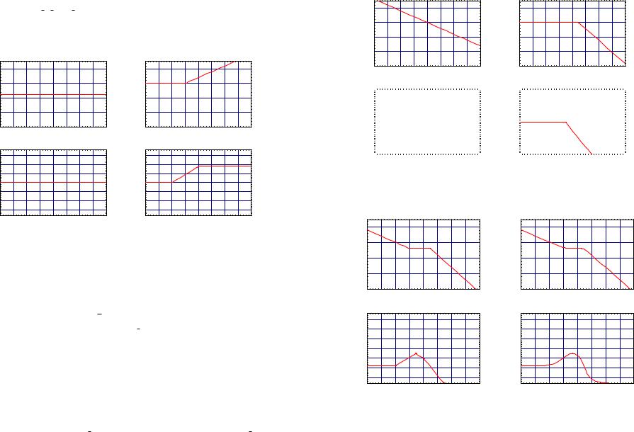
1. H(ω) = K: The Bode plot here is simple. It takes the magnitude 20 log K for all values of log ω. The phase is 0◦ for all log ω if K is positive, and 180◦ otherwise.

2.H(ω) = 1 + iωτ: For ω near zero the frequency response looks like 1 and so has the value of 0dB. For large ω the frequency response looks like iωτ, and so the log of the

magnitude will look like log ωτ. Thus the magnitude plot for large frequencies we have |H(ω)| ≈ 20 log ωτdB. These asymptotes meet when 20 log ωτ = 0 or when ω = τ1 . This point is called the break frequency. Note that the slope of the frequency response for large ω is independent of τ (since log ωτ = log ω + log τ), but its break frequency does depend on τ. The phase plot starts at 0 for ω small and for large ω, since the frequency response is predominantly imaginary, becomes 90◦. This Bode plot is shown in Figure 4.6 for τ = 1.

3. H(ω) = 1 + 2iζ

ω

− (

ω 2

)

: For small ω the magnitude is 1 or 0dB. For large ω the

ω0

ω0

frequency response looks like −ω(

ω

2

ω

)

and so the magnitude looks like 40 log

. The two

ω0

ω0

asymptotes meet when

40 log

= 0 or when ω = ω0. One has to be a bit more careful

ω0

with what is happening around the frequency ω0. The behaviour here depends on the value of ζ, and various plots are shown in Figure 4.6 for ω0 = 1. As ζ decreases, the undershoot increases. The phase starts out at 0◦ and goes to 180◦ as ω increases.

4.H(ω) = (iω)−1: The magnitude is ω1 over the entire frequency range which gives |H(ω)| = −20 log ωdB. The phase is −90◦ over the entire frequency range, and the simple Bode plot is shown in Figure 4.7.

5.H(ω) = (1 + iωτ)−1: The analysis here is just like that for a real zero except for signs. The Bode plot is shown in for τ = 1.

	ω		ω
6. H(ω) = (1 + 2iζ		− (		)2)−1: The situation here is much like that for a complex zero
	ω0		ω0

with sign reversal. The Bode plots are shown in Figure 4.8 for ω0 = 1.

4.8 Remark We note that one often sees the language “20dB/decade.” With what we have done above for the typical elements in a frequency response function. A first-order element in the numerator increases like 20 log τω for large frequencies. Thus as ω increases by a factor of 10, the magnitude will increase by 20dB. This is where “20dB/decade” comes from. If the first-order element is in the denominator, then the magnitude decreases at 20dB/decade. Second-order elements in the numerator increase at 40dB/decade, and second-order elements in the denominator decrease at 40dB/decade. In this way, one can ascertain the relative

22/10/2004

4.3 Graphical representations of the frequency response

131

	40							40
	30							30
	20							20
dB	10						dB	10
	0							0
	-10							-10
	-20							-20
	-30							-30
	-1.5 -1 -0.5	0	0.5	1	1.5	2		-1.5 -1 -0.5	0	0.5	1	1.5	2

log ω

log ω

	150							150
	100							100
deg	50						deg	50
	0							0
	-50							-50
	-100							-100
	-150							-150
	-1.5 -1 -0.5	0	0.5	1	1.5	2		-1.5 -1 -0.5	0	0.5	1	1.5	2

log ω log ω

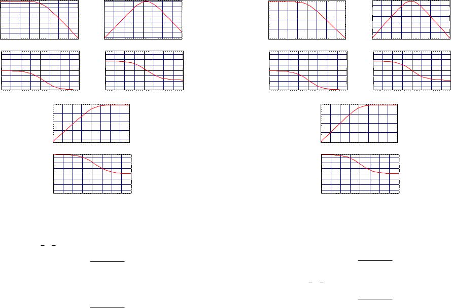
Figure 4.6 Bode plot for H(ω) = 1 + iω (left) and for H(ω) = 1 + 2iζω − ω2 for ζ = 0.2, 0.4, 0.6, 0.8 (right)

	40						40
	30						30
	20						20
dB	10					dB	10
	0						0
	-10						-10
	-20						-20
	-30						-30
	-1.5 -1 -0.5	0	0.5	1	1.5	2

log ω

-1.5 -1 -0.5

0

0.5

1

1.5

2

log ω

	150							150
	100							100
deg	50						deg	50
	0							0
	-50							-50
	-100							-100
	-150							-150
	-1.5 -1 -0.5	0	0.5	1	1.5	2		-1.5 -1 -0.5	0	0.5	1	1.5	2

log ω

log ω

Figure 4.7 Bode plot for H(ω) = (iω)−1 (left) and for H(ω) = (1 + iω)−1 (right)

132

4 Frequency response (the frequency domain)

22/10/2004

	40
	30
	20
dB	10
	0
	-10
	-20
	-30
	-1.5 -1 -0.5	0	0.5	1	1.5	2

log ω

	150
	100
deg	50
	0
	-50
	-100
	-150
	-1.5 -1 -0.5	0	0.5	1	1.5	2

log ω

Figure 4.8 Bode plot for H(ω) = (1 + 2iζω − ω2)−1 for ζ = 0.2, 0.4, 0.6, 0.8

degree of the numerator and denominator of a frequency response function by looking at its slope for large frequencies. Indeed, we have the following rule:

The slope of the magnitude Bode plot for HN,D at large frequencies is 20(deg(N)− deg(D))dB/decade.

To get a rough idea of how to sketch a Bode plot, the above arguments illustrate that the asymptotes are the most essential feature. Thus we illustrate these asymptotes in Figure 4.19 (see the end of the chapter) for the essential Bode plots in the above list. From these one can determine the character of most any Bode plot. The reason for this is that in (4.3) we have ensured that any frequency response is a product of the factors we have individually examined. Thus when we take logarithms as we do when generating a Bode plot, the graphs simply add! And the same goes for phase plots. So by plotting each term individually by the above rules, we end up with a pretty good rough approximation by adding the Bode plots.

Let us illustrate how this is done in an example.

4.9 Example (Example 4.7 cont’d) We take the frequency response

	1		1 + i10ω
H(ω) =				.
	80		iω 1 + 2i√12 √ω8 − (√ω8 )2

Four essential elements will comprise the frequency response:

1.H1(ω) = 801 ;

2.H2(ω) = 1 + i10ω;

22/10/2004		4.3 Graphical representations of the frequency response									133
3.	H3(ω) = (iω)−1;
4.		1	ω		ω		2		−1	.
	H4(ω) = 1 + 2i√2		√8	− (√8 )
Let’s look first		at the magnitudes.
1.	H1 will contribute 20 log				1		≈ −38.1dB. The asymptotes for H1 are shown in Fig-
					80
	ure 4.9.

	50		50
	0		0
dB	-50	dB	-50
	-100		-100
	-3 -2 -1 0 1 2 3 4		-3 -2 -1 0 1 2 3 4

log ω

log ω

		150		150
		100		100
	deg	50	deg	50
		0		0
		-50		-50
		-100		-100
		-150		-150
		-3 -2 -1 0 1 2 3 4		-3 -2 -1 0 1 2 3 4

log ω		log ω
Figure 4.9 Asymptotes for Example 4.7: H1 (left) and H2 (right)
2. H2 has a break frequency of ω =	1	or log ω = −1. The asymptotes for H2 are shown
	10
in Figure 4.9.

3. H3 gives −20 log ω across the board. The asymptotes for H3 are shown in Figure 4.10.

√

4. H4 has a break frequency of ω = 8 or log ω ≈ 0.45. The asymptotes for H4 are shown

in Figure 4.10. Note that here we have ζ = 1 , which is a largish value. Thus we do

√

2

not need to adjust the magnitude peak too much around the break frequency when we use the asymptotes to approximate the actual Bode plot.

Now the phase angles.

1.H1 has phase exactly 0 for all frequencies.

2.For H2, the phase is approximately 0◦ for log 10ω < −1 or log ω < −2. For log 10ω > 1

(or log ω > 0) the phase is approximately 90◦. Between the frequencies log ω =

−

2

and log ω = 0 we interpolate linearly between the two asymptotic phase angles.

3.

The phase for H3 is −90◦ for all frequencies.

√

ω

ω

4.

For H4, the phase is 0◦ for log √8 < −1 or log ω < log

8 −1 ≈ −0.55. For log √8

> 1,

≈

−

(log ω > log √8 + 1

1.45), the phase is approximately

180◦.

134

4 Frequency response (the frequency domain)

22/10/2004

	50		50
	0		0
dB	-50	dB	-50
	-100		-100
		-3 -2 -1 0 1 2 3 4

log ω

-3 -2 -1 0 1 2 3 4

log ω

	150											150
	100											100
deg	50										deg	50
	0											0
	-50											-50
	-100											-100
	-150											-150
		-3 -2 -1 0 1 2 3 4										-3 -2 -1 0 1 2 3 4
				log ω											log ω

Figure 4.10 Asymptotes for Example 4.7: H3 (left) and H4 (right)

	50		50
	0		0
dB	-50	dB	-50
	-100		-100
		-3 -2 -1 0 1 2 3 4

log ω

-3 -2 -1 0 1 2 3 4

log ω

		150		150
		100		100
	deg	50	deg	50
		0		0
		-50		-50
		-100		-100
		-150		-150
		-3 -2 -1 0 1 2 3 4		-3 -2 -1 0 1 2 3 4

log ω

log ω

Figure 4.11 The sum of the asymptotes (left) and the actual Bode plot (right) for Example 4.7

22/10/2004 4.4 Properties of the frequency response 135

The sum of the asymptotes are plotted in Figure 4.11 along with the actual Bode plot so you can see how the Bode plot is essentially the sum of the individual Bode plots. You should take care that you always account for ζ, however. In our example, the value of ζ in H4 is

quite large, so not much of an adjustment had to be made. If ζ were small, we have to add

√

a little bit of a peak in the magnitude around the break frequency log ω = log 8, and also

make the change in the phase a bit steeper.
4.3.3 The polar frequency response plot	We will encounter in Chapter 12 another

representation of the frequency response H. The idea here is that rather than plotting magnitude and phase as one does in a Bode plot, one plots the real and imaginary part of the frequency response as a curve in the complex plane parameterised by ω (0, ∞). Doing this yields the polar plot for the frequency response. One could do this, for example, by taking the Bode plot, and for each point ω on the independent variable axis, put a point at a distance |H(ω)| from the origin in the direction ]H(ω). Indeed, given the Bode plot, one can typically make a pretty good approximation of the polar plot by noting (1) the maxima and minima of the magnitude response, and the phase at these maxima and minima, and

(2)the magnitude when the phase is 0, ±90◦, or ±180◦.

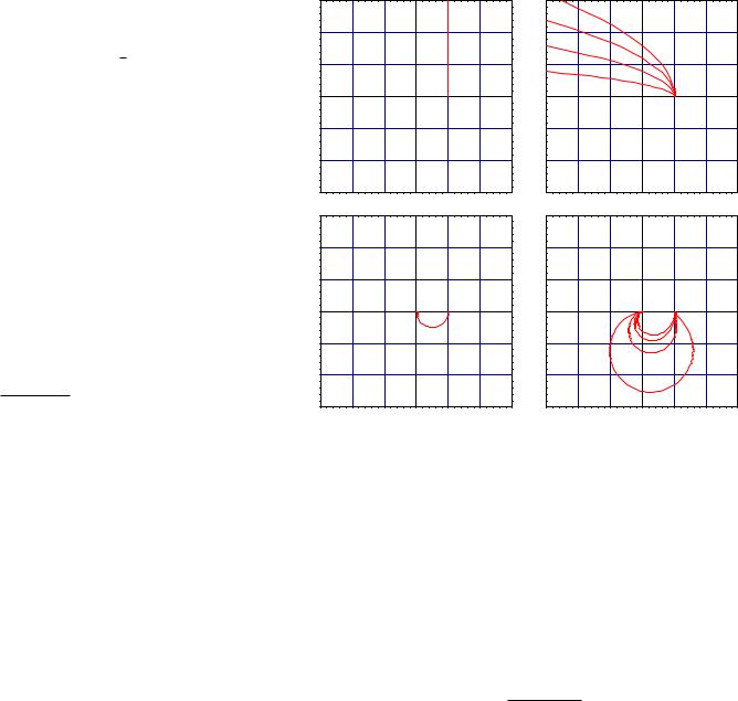
In Figure 4.12 are shown the polar plots for the basic frequency response functions.

Recall that in (4.3) we indicated that any frequency response will be a product of these basic elements, and so one can determine the polar plot for a frequency response formed by the product of such elements by performing complex multiplication that, you will recall, is done in polar coordinates merely by multiplying radii, and adding angles.

For a lark, let’s look at the minimum/nonminimum phase example in polar form.

4.10 Example (Example 4.12) Recall that we contrasted the two transfer functions

HΣ1 (ω) =	1 + iω	, HΣ2 (ω) =	1 − iω	.
	−ω2 + iω + 1
			−ω2 + iω + 1

We contrast the polar plots for these frequency responses in Figure 4.13. Note that, as expected, the minimum phase system undergoes a smaller phase change if we follow it along its parameterised polar curve. We shall see the potential dangers of this in Chapter 12.

Note that when making a polar plot, the thing one looses is frequency information. That is, one can no longer read from the plot the frequency at which, say, the magnitude of the frequency response is maximum. For this reason, it is not uncommon to place at intervals along a polar plot the frequencies corresponding to various points.

4.4 Properties of the frequency response

It turns out that in the frequency response can be seen some of the behaviour we have encountered in the time-domain and in the transfer function. We set out in this section to scratch the surface behind interpreting the frequency response. However, this is almost an art as much as a science, so plain experience counts for a lot here.

4.4.1 Time-domain behaviour reflected in the frequency response We have seen in Section 3.2 we saw that some of the time-domain properties discussed in Section 2.3 were reflected in the transfer function. We anticipate being able to see these same features

136		4 Frequency response (the frequency domain)											22/10/2004
	3							3
	2							2
	1							1
Im	0						Im	0
	-1							-1
	-2							-2
	-2	-1	0	1	2	3			-2	-1	0	1	2	3
			Re								Re
	3							3
	2							2
	1							1
Im	0						Im	0
	-1							-1
	-2							-2
	-2	-1	0	1	2	3			-2	-1	0	1	2	3
			Re								Re
		Figure 4.12 Polar plots for H(ω)					= 1 + iω (top left),				H(ω)	=
		1 + 2iζω − ω2, ζ			= 0.2, 0.4, 0.6, 0.8				(top	right),	H(ω)	=
		(1 + iω)−1		(bottom left),		and H(ω)			= (1 + 2iζω − ω2)−1,

ζ = 0.2, 0.4, 0.6, 0.8

reflected in the frequency response, and ergo in the Bode plot. In this section we explore these expected relationships. We do this by looking at some examples.

4.11 Example The first example we look at is one where we have a pole/zero cancellation. As per Theorem 3.5 this indicates a lack of observability in the system. It is most beneficial to look at what happens when the pole and zero do not actually cancel, and compare it to what happens when the pole and zero really do cancel. We take

A =	1	−	,	b =	1	,	c =	1	,	(4.4)
	0	1			0			1

and we compute

1 + iω

HΣ(ω) = −ω2 + i ω − 1.

22/10/2004			4.4	Properties of the frequency response							137
	1						1
	0.5						0.5
	0						0
Im	-0.5					Im	-0.5
	-1						-1
	-1.5						-1.5
	-1 -0.5	0	0.5	1	1.5		-1 -0.5	0	0.5	1	1.5
		Re						Re

Figure 4.13 Polar plots for minimum phase (left) and nonminimum phase (right) systems

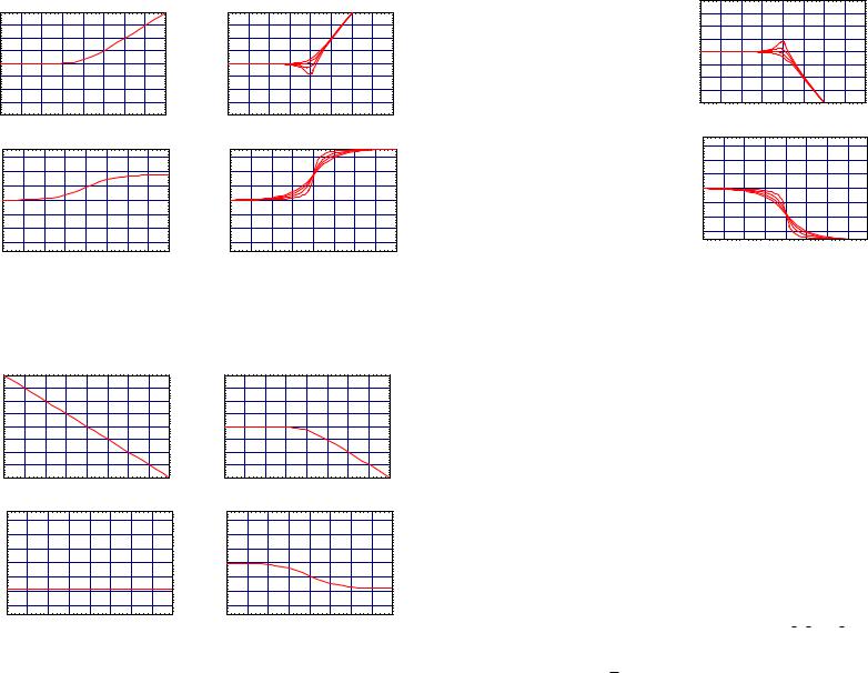
The Bode plots for three values of are shown in Figure 4.14. What are the essential features here? Well, by choosing the values of 6= 0 to deviate significantly from zero, we can see accentuated two essential points. Firstly, when 6= 0 the magnitude plot has two regions where the magnitude drops o at di erent slopes. This is a consequence of there being two di erent exponents in the characteristic polynomial. When = 0 the plot tails o at one slope, indicating that the system is first-order and has only one characteristic exponent. This is a consequence of the pole/zero cancellation that occurs when = 0. Note, however, that we cannot look at one Bode plot and ascertain whether or not the system is observable.

There is also an e ect that can be observed in the Bode plot for a system that is not minimum phase. An example illustrates this well.

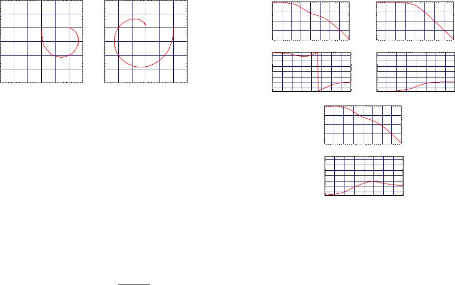
4.12 Example We consider two SISO linear systems, both with

A =	−1		−1	,		b =	1 .	(4.5)
		0	1				0
The two output vectors we look at are		1				−1 .
c1	=		, c2		=			(4.6)
		1				1

Let us then denote Σ1 = (A, b, c1, 01) and Σ2 = (A, b, c2, 01). The two frequency response functions are

HΣ1 (ω) =	1 + iω	, HΣ2 (ω) =	1 − iω	.
	−ω2 + iω + 1
			−ω2 + iω + 1

The Bode plots are shown in Figure 4.15. What should one observe here? Note that the magnitude plots are the same, and this can be verified by looking at the expressions for HΣ1 and HΣ2 . The di erences occur in the phase plots. Note that the phase angle varies only slightly for Σ1 across the frequency range, but it varies more radically for Σ2. It is from this behaviour that the term “minimum phase” is derived.

138

4 Frequency response (the frequency domain)

22/10/2004

0
-10
dB-20
-30
-40	-1	-0.5	0	0.5	1	1.5	2
-1.5

log ω

0
-10
dB-20
-30
-40	-1	-0.5	0	0.5	1	1.5	2
-1.5

log ω

	150									150
	100									100
deg	50								deg	50
	0									0
	-50									-50
	-100									-100
	-150									-150
	-1.5	-1	-0.5	0	0.5	1	1.5	2		-1.5	-1	-0.5	0	0.5	1	1.5	2

log ω

log ω

0
-10
dB-20
-30
-40	-1	-0.5	0	0.5	1	1.5	2
-1.5

log ω

	150
	100
deg	50
	0
	-50
	-100
	-150
	-1.5	-1	-0.5	0	0.5	1	1.5	2

log ω

Figure 4.14 Bode plots for (4.4) for = −5, = 0, and = 5

4.4.2 Bode’s Gain/Phase Theorem In Bode’s book [1945] one can find a few chapters on some properties of the frequency response. In this section we begin this development, and from it derive Bode’s famous “Gain/Phase Theorem.” The material in this section relies on some ideas from complex function theory

that we review in Appendix D. We start by examining some basic properties of frequency response functions. Here we begin to see that the real and imaginary parts of a frequency response function are not arbitrary functions.

4.13 Proposition Let (N, D) be a SISO linear system in input/output form with HN,D the frequency response. The following statements hold:

(i)Re(HN,D(−ω)) = Re(HN,D(ω));

(ii)Im(HN,D(−ω)) = −Im(HN,D(ω));

(iii)|HN,D(−ω)| = |HN,D(ω)|;