6.PID control

Chapter 6. PID Control

uncertainty. When this is done the response to set points can be adjusted by choosing the parameters b and c. The controller parameters appear in a much more complicated way in the PIPD controller.

6.5 Windup

Although many aspects of a control system can be understood based on linear theory, some nonlinear effects must be accounted for in practically all controllers. Windup is such a phenomena, which is caused by the interaction of integral action and saturations. All actuators have limitations: a motor has limited speed, a valve cannot be more than fully opened or fully closed, etc. For a control system with a wide range of operating conditions, it may happen that the control variable reaches the actuator limits. When this happens the feedback loop is broken and the system runs as an open loop because the actuator will remain at its limit independently of the process output. If a controller with integrating action is used, the error will continue to be integrated. This means that the integral term may become very large or, colloquially, it “winds up”. It is then required that the error has opposite sign for a long period before things return to normal. The consequence is that any controller with integral action may give large transients when the actuator saturates. We will illustrate this by an example.

EXAMPLE 6.2—ILLUSTRATION OF INTEGRATOR WINDUP

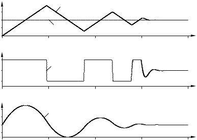
The wind-up phenomenon is illustrated in Figure 6.6, which shows control of an integrating process with a PI controller. The initial setpoint change is so large that the actuator saturates at the high limit. The integral term increases initially because the error is positive; it reaches its largest value at time t 10 when the error goes through zero. The output remains saturated at this point because of the large value of the integral term. It does not leave the saturation limit until the error has been negative for a sufficiently long time to let the integral part come down to a small level. Notice that the control signal bounces between its limits several times. The net effect is a large overshoot and a damped oscillation where the control signal flips from one extreme to the other as in relay oscillation. The output finally comes so close to the setpoint that the actuator does not saturate. The system then behaves linearly and settles.

The example show integrator windup which is generated by a change in the reference value. Windup may also be caused by large disturbances or equipment malfunctions. It can also occur in many other situations.

The phenomenon of windup was well known to manufacturers of analog controllers who invented several tricks to avoid it. They were described

226

6.5 Windup

	2		y
	1
	0		ysp
		20	40	60	80
	0
	0.1		u
	−0.1
	0	20	40	60	80
	2		I
	−2
	0	20	40	60	80

Figure 6.6 Illustration of integrator windup. The diagrams show process output y, setpoint ysp, control signal u, and integral part I.

under labels like preloading, batch unit, etc. Although the problem was well understood, there were often restrictions caused by the analog technology. The ideas were often kept as trade secrets and not much spoken about. The problem of windup was rediscovered when controllers were implemented digitally and several methods to avoid windup were presented in the literature. In the following section we describe some of the methods used to avoid windup.

Setpoint Limitation

One attempt to avoid integrator windup is to introduce limiters on the setpoint variations so that the controller output never reaches the actuator limits. This frequently leads to conservative bounds and poor performance. Furthermore, it does not avoid windup caused by disturbances.

Incremental Algorithms

In the early phases of feedback control, integral action was integrated with the actuator by having a motor drive the valve directly. In this case windup is handled automatically because integration stops when the valve stops. When controllers were implemented by analog techniques,

227

Chapter 6. PID Control

–y

KTds

Actuator

model

Actuator

e = r − y

Σ

K

–

+

K

Σ

1

Σ

Ti

s

es

1

Tt

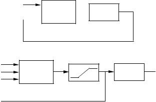
Figure 6.7 Controller with anti-windup where the actuator output is estimated from a mathematical model.

and later with computers, many manufacturers used a configuration that was an analog of the old mechanical design. This led to the so-called velocity algorithms. A velocity algorithm first computes the rate of change of the control signal which is then fed to an integrator. In some cases this integrator is a motor directly connected to the actuator. In other cases the integrator is implemented internally in the controller. With this approach it is easy to avoid windup by inhibiting integration whenever the output saturates. This method is equivalent to back-calculation, which is described below. If the actuator output is not measured, a model that computes the saturated output can be used. It is also easy to limit the rate of change of the control signal.

Back-Calculation and Tracking

Back-calculation works as follows: When the output saturates, the integral term in the controller is recomputed so that its new value gives an output at the saturation limit. It is advantageous not to reset the integrator instantaneously but dynamically with a time constant Tt.

Figure 6.7 shows a block diagram of a PID controller with anti-windup based on back-calculation. The system has an extra feedback path that is generated by measuring the actual actuator output and forming an error signal DesE as the difference between the output of the controller DvE and the actuator output DuE. Signal es is fed to the input of the integrator through gain 1/Tt. The signal is zero when there is no saturation. Thus, it will not have any effect on the normal operation when the actuator does not saturate. When the actuator saturates, the signal es is different from zero. The normal feedback path around the process is broken because the

228

6.5 Windup

ysp

1

0.5y

0	10	20	30
0
0.15
0.05		u
−0.05	10	20	30
0
0
−0.4	I
−0.8	10	20	30
0

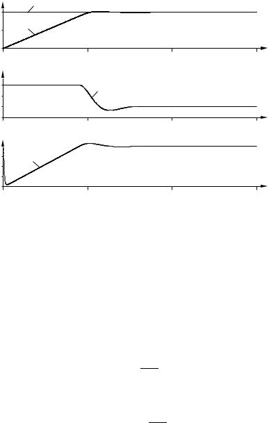
Figure 6.8 Controller with anti-windup applied to the system of Figure 6.6. The diagrams show process output y, setpoint ysp, control signal u, and integral part I.

process input remains constant. There is, however, a feedback path around the integrator. Because of this, the integrator output is driven towards a value such that the integrator input becomes zero. The integrator input is

1	es	K	e
Tt		Ti

where e is the control error. Hence,

es − K Tt e Ti

in steady state. Since es u − v, it follows that

K Tt v ulim Ti e

where ulim is the saturating value of the control variable. This means that the signal v settles on a value slightly out side the saturation limit and the control signal can react as soon as the error changes time. This prevents

229

Chapter 6.	PID Control
	ysp	Tt 3
1		Tt 2
		Tt 0.1, Tt 1
0	10	20	30
0
0.1	Tt 0.1	Tt 3
0		Tt 2
	Tt 1
−0.1
0	10	20	30

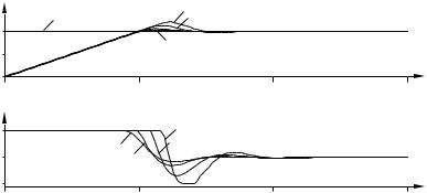
Figure 6.9 The step response of the system in Figure 6.6 for different values of the tracking time constant Tt. The upper curve shows process output y and setpoint ysp, and the lower curve shows control signal u.

the integrator from winding up. The rate at which the controller output is reset is governed by the feedback gain, 1/Tt, where Tt can be interpreted as the time constant, which determines how quickly the integral is reset. We call this the tracking time constant.

It frequently happens that the actuator output cannot be measured. The anti-windup scheme just described can be used by incorporating a mathematical model of the saturating actuator, as is illustrated in Figure 6.7.

Figure 6.8 shows what happens when a controller with anti-windup is applied to the system simulated in Figure 6.6. Notice that the output of the integrator is quickly reset to a value such that the controller output is at the saturation limit, and the integral has a negative value during the initial phase when the actuator is saturated. This behavior is drastically different from that in Figure 6.6, where the integral has a positive value during the initial transient. Also notice the drastic improvement in performance compared to the ordinary PI controller used in Figure 6.6.

The effect of changing the values of the tracking time constant is illustrated in Figure 6.9. From this figure, it may thus seem advantageous to always choose a very small value of the time constant because the integrator is then reset quickly. However, some care must be exercised when introducing anti-windup in systems with derivative action. If the time constant is chosen too small, spurious errors can cause saturation of the output, which accidentally resets the integrator. The tracking time constant Tt should be larger than Td and smaller than Ti. A rule of thumb

230

6.5 Windup

y sp

b

Σ

K

P

y

D

−1

sKTd

Σ

e

1+ sTd / N

I

K

Σ

1

Σ

v

Ti

s

1

Tt

w

+

–

y sp

Σ

SP

v

y

MV

PID

w

TR

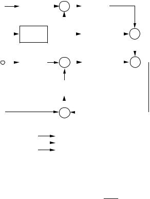
Figure 6.10 Block diagram and simplified representation of PID module with tracking signal.

T that has been suggested is to choose Tt TiTd.

Controllers with a Tracking Mode

A controller with back-calculation can be interpreted as having two modes: the normal control mode, when it operates like an ordinary controller, and a tracking mode, when the controller is tracking so that it matches given inputs and outputs. Since a controller with tracking can operate in two modes, we may expect that it is necessary to have a logical signal for mode switching. However, this is not necessary, because tracking is automatically inhibited when the tracking signal w is equal to the controller output. This can be used with great advantage when building up complex systems with selectors and cascade control.

Figure 6.10 shows a PID module with a tracking signal. The module has three inputs: the setpoint, the measured output, and a tracking signal. The new input TR is called a tracking signal because the controller output will follow this signal. Notice that tracking is inhibited when w v. Using the module the system shown in Figure 6.7 can be presented as shown in Figure 6.11.

231

Chapter 6. PID Control

A

SP

MV PID Actuator

TR

			B
			Actuator model
	SP	v	u
	MV			Actuator
		PID
	TR

Figure 6.11 Representation of the controllers with anti-windup in Figure 6.7 using the basic control module with tracking shown in Figure 6.10.

6.6 Tuning

All general methods for control design can be applied to PID control. A number of special methods that are tailor-made for PID control have also been developed, these methods are often called tuning methods. Irrespective of the method used it is essential to always consider the key elements of control, load disturbances, sensor noise, process uncertainty and reference signals.

The most well known tuning methods are those developed by Ziegler and Nichols. They have had a major influence on the practice of PID control for more than half a century. The methods are based on characterization of process dynamics by a few parameters and simple equations for the controller parameters. It is surprising that the methods are so widely referenced because they give moderately good tuning only in restricted situations. Plausible explanations may be the simplicity of the methods and the fact that they can be used for simple student exercises in basic control courses.

The Step Response Method

One tuning method presented by Ziegler and Nichols is based on a process information in the form of the open-loop step response obtained from a bump test. This method can be viewed as a traditional method based on modeling and control where a very simple process model is used. The step response is characterized by only two parameters a and L, as shown in

232

6.6 Tuning

Figure 6.12 Characterization of a step response in the Ziegler-Nichols step response method.

Table 6.1 PID controller parameters obtained for the Ziegler-Nichols step response method.

Controller	K	Ti	Td	Tp
P	1/a			4L
PI	0.9/a	3L	L/2	5.7L
PID	1.2/a	2L		3.4L

Figure 6.12.

The point where the slope of the step response has its maximum is first determined, and the tangent at this point is drawn. The intersections between the tangent and the coordinate axes give the parameters a and L. The controller parameters are then obtained from Table 6.1. An estimate of the period Tp of the closed-loop system is also given in the table.

The Frequency Response Method

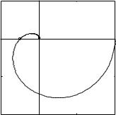
A second method developed by Ziegler and Nichols is based on a simple characterization of the the frequency response of the process process dynamics. The design is based on knowledge of only one point on the Nyquist curve of the process transfer function PDsE, namely the point where the Nyquist curve intersects the negative real axis. This point can be characterized by two parameters the frequency ω 180 and the gain at that frequency k180 hPDiω 180Eh. For historical reasons the point has been called the ultimate point and characterized by the parameters Ku 1/K180 and Tu 2π /ω 180, which are called the ultimate gain and the ultimate period. These parameters can be determined in the following way. Connect a controller to the process, set the parameters so that control action is proportional, i.e., Ti [ and Td 0. Increase the gain slowly until the

233

Chapter 6. PID Control

0.5
0
−0.5
−1	0	0.5	1
−0.5

Figure 6.13 Characterization of a step response in the Ziegler-Nichols step response method.

Table 6.2 Controller parameters			for the	Ziegler-Nichols			frequency response
method.
	Controller	K	Ti		Td		Tp
	P	0.5Ku					Tu
	PI	0.4Ku	0.8Tu				1.4Tu
	PID	0.6Ku	0.5Tu		0.125Tu		0.85Tu

process starts to oscillate. The gain when this occurs is Ku and the period of the oscillation is Tu. The parameters of the controller are then given by Table 6.2. An estimate of the period Tp of the dominant dynamics of the closed-loop system is also given in the table.

The frequency response method can be viewed as an empirical tuning procedure where the controller parameters are obtained by direct experiments on the process combined with some simple rules. For a proportional controller the rule is simply to increase the gain until the process oscillates and then reduce it by 50%.

Assessment of the Ziegler Nichols Methods

The Ziegler-Nichols tuning rules were developed to give closed loop systems with good attenuation of load disturbances. The methods were based on extensive simulations. The design criterion was quarter amplitude decay ratio, which means that the amplitude of an oscillation should be reduced by a factor of four over a whole period. This corresponds to closed loop poles with a relative damping of about ζ 0.2, which is too small.

234

6.6 Tuning

Controllers designed by the Ziegler-Nichols rules thus inherently give closed loop systems with poor robustness. It also turns out that it is not sufficient to characterize process dynamics by two parameters only. The methods developed by Ziegler and Nichols have been been very popular in spite of these drawbacks. Practically all manufacturers of controller have used the rules with some modifications in recommendations for controller tuning. One reason for the popularity of the rules is that they are simple and easy to explain. The tuning rules give ball park figures. Final tuning is then done by trial and error. Another DbadE reason is that the rules lend themselves very well to simple exercises for control education.

With the insight into controller design that has developed over the years it is possible to develop improved tuning rules that are almost as simple as the Zigler-Nichols rules. These rules are developed by starting with a solid design method that gives robust controllers with effective disturbance attenuation. We illustrate with some rules where the process is characterized by three parameters.

An Improved Step Response Method

This method characterizes the unit step response by three parameters K , L and T for stable processes and K v K /T and L for integrating processes. This parameterization matches the transfer functions

			kp
P1DsE				e−sL
		1 sT
P s	E	kv	e−sL
2D		s

The transfer function P1DsE, which is called a first order system with time delay or a K LT model. Parameter L is determined from the intercept of the tangent with largest slope with the time axis as was described in Figure 6.12. Parameter T is also determined as shown in the figure as the difference between the time when the step response reaches 63% of its steady state value. Parameter kp is the static gain of the system. The parameter kv is the largest slope of the unit step response. Parameter L is called the apparent time delay and parameter T the apparent time constant or the apparent lag. The adverb apparent is added to indicate that parameters are based on approximations. The parameter

τ	L
	L T

is called the relative time delay. This parameter is a good indicator of process dynamics.

235