Alvord L.Easy J.2002

For the purposes of display, it is often convenient to use a verb transpose |: which reorganises a list of lists into a new set of lists in which the first list is a list of all first items, the second list is a list of all second items and so on :

|:#:i.8

0 0 0 0 1 1 1 1

0 0 1 1 0 0 1 1

0 1 0 1 0 1 0 1

Thus, returning to the pizza problem, given 0 means absent and 1 means present

|:#:i.16

0 0 0 0 0 0 0 0 1 1 1 1 1 1 1 1

0 0 0 0 1 1 1 1 0 0 0 0 1 1 1 1

0 0 1 1 0 0 1 1 0 0 1 1 0 0 1 1

0 1 0 1 0 1 0 1 0 1 0 1 0 1 0 1

represents all the possible choices of toppings.

There is no requirement that all the items in the left argument of dyadic #: are the same. If we wished to allow three possibilities for the second row, say because two types of cheese become available making a total of 24 possible pizzas in total, we can supply 2 3 2 2 as the left argument :

|:2 3 2 2#:i.24

0 0 0 0 0 0 0 0 0 0 0 0 1 1 1 1 1 1 1 1 1 1 1 1

0 0 0 0 1 1 1 1 2 2 2 2 0 0 0 0 1 1 1 1 2 2 2 2

0 0 1 1 0 0 1 1 0 0 1 1 0 0 1 1 0 0 1 1 0 0 1 1

0 1 0 1 0 1 0 1 0 1 0 1 0 1 0 1 0 1 0 1 0 1 0 1

Now the 24 is just the product of 2 3 2 and 2, or in J terminology */2 3 2 2, and so there is some redundancy in the above expression. J allows us to avoid this by using a hook with #: as the left verb, and i.@(*/) as the right verb :

poss=.#:i.@(*/) |: poss 2 3 2 2

0 0 0 0 0 0 0 0 0 0 0 0 1 1 1 1 1 1 1 1 1 1 1 1

0 0 0 0 1 1 1 1 2 2 2 2 0 0 0 0 1 1 1 1 2 2 2 2

0 0 1 1 0 0 1 1 0 0 1 1 0 0 1 1 0 0 1 1 0 0 1 1

0 1 0 1 0 1 0 1 0 1 0 1 0 1 0 1 0 1 0 1 0 1 0 1

Now make and display a list of the ingredients, using open and link described in section 5 :

]tops=.>'onions';'cheese';'sausage';'mushrooms ' onions

cheese sausage mushrooms

30

The leftmost verb right ], by virtue of its definition, causes a display of everything to its right. Earlier monadic + and , were used for this purpose; in practice right is much the commonest way of doing simultaneous assignment and display because it is independent of type (character or numeric). Now define

tab=.|:poss 2 3 2 2 tops,tab

|domain error

| tops ,tab

The problem here is that J does not allow mixed types (character and numeric) to be appended. However, J does provide a very convenient verb format ": which transforms any numeric object into its character equivalent which looks identical on display :

tops,":tab onions cheese sausage mushrooms

0 0 0 0 0 0 0 0 0 0 0 0 1 1 1 1 1 1 1 1 1 1 1 1

0 0 0 0 1 1 1 1 2 2 2 2 0 0 0 0 1 1 1 1 2 2 2 2

0 0 1 1 0 0 1 1 0 0 1 1 0 0 1 1 0 0 1 1 0 0 1 1

0 1 0 1 0 1 0 1 0 1 0 1 0 1 0 1 0 1 0 1 0 1 0 1

Not quite what we were thinking of - what is needed is append items ,. which was first met in section 4, and is now used to append the two lists on an item by item basis as opposed to one list after the other. At the same time we have incorporated the dyadic form of format which allows a field size to be specified, in this case 1 :

tops,.1 ":tab

onions 000000000000111111111111 cheese 000011112222000011112222 sausage 001100110011001100110011 mushrooms 010101010101010101010101

Now suppose that we want to compute the costs of the various types of pizza, given the costs of the various toppings :

cost=.0.80 1.80 2.20 1.50

The required calculation is to multiply each of the four lists (rows) in tab by the matching element in cost and then add “down the columns”, that is a +/ applied to each column. This combination of addition and multiplication, sometimes known as an “inner product” is expressed by the dot conjunction, and so

cost +/ .* tab

0 1.5 2.2 3.7 1.8 3.3 4 5.5 3.6 5.1 5.8 7.3 0.8 2.3 3 4.5

2.6 4.1 4.8 6.3 4.4 5.9 6.6 8.1

31

gives a list of the 24 possible pizzas.

To display the combinations in the form of a price list use format once again, only now applying it dyadically to specify a field width of 1 with no decimals for the first four columns, and 6 with 2 decimal places for the price column :

((4#1j0),6j2)":|:tab,cost +/ .* tab 0000 0.00 0001 1.50 0010 2.20 0011 3.70 0100 1.80 0101 3.30 0110 4.00 0111 5.50

…………….. ..

…

and so on. The leftmost column is not very informative, so use copy to make it more meaningful, having first used append items monadically to change it from a list of 24 items to a list of 24 single-item lists :

$prices=.cost+/ .*tab

24

$,.prices

241

((|:tab)#'OCSM'),.6j2":,.prices

M	0.00
	1.50
S	2.20
SM	3.70
C	1.80
CM	3.30
CS	4.00
CSM	5.50
CC	3.60
CCM	5.10
CCS	5.80
CCSM	7.30
O	0.80
OM	2.30
OS	3.00
OSM	4.50
OC	2.60
OCM	4.10
OCS	4.80
OCSM	6.30
OCC	4.40
OCCM	5.90
OCCS	6.60
OCCSM	8.10

32

SECTION 7 : EDITING, SYSTEM FACILITIES and SCRIPTS

Sooner or later you will want to write “programs” which you cannot express on a single line. While J contains many sophisticated features which make it possible to express a great deal in a single phrase, it can be comforting to know that a more conventional style of conditional and looping programming is also available. We look at three ways in which a user-defined verb for Fibonacci numbers can be constructed. Fibonacci numbers are sequences which are started with two arbitrary numbers (most commonly 0 and 1), and thereafter each succeeding number is the sum of the previous two. Clearly such a series could go on indefinitely, and so for practical purposes one of the parameters of a Fibonacci verb must provide a stopping condition, for example, either a total number of numbers is given, or the series may stop after a given value has been exceeded.

The English of the previous sentence can be rendered in J as _2&{. (take the last two) and then +/@(_2&{.) (sum the last two). Finally we want to join this to what we started with, which is the verb structure previously recognised as a hook ,+/@(_2&{.) . Hence a user-defined verb for a single Fibonacci step is

fib=.,+/@(_2&{.) fib 2 3

2 3 5

Suppose that the stopping condition is that this step has to be performed a given number of times, say 10. J provides a conjunction power ^: which allows us to say just this. Its symbol demonstrates the analogy with the power verb which prescribes how often a number is to be multiplied by itself.

0	1	fib^:10(0 1)					21 34	55	89
		1	2	3 5	8	13

We can even write this series all in a single line without any named verb, although the expression could be criticised as becoming a little bit hard to disentangle :

(,+/@(_2&{.))^:10(0 1)

0 1 1 2 3 5 8 13 21 34 55 89

Next, here, side by side, are two alternative ways in which we could have written and executed this program, the second shows incidentally that J supports recursion :

Fib=.dyad define									Fib=.dyad define
r=.y. [ i=.0									if.x.>0 do.
while. i<x. do.									r=.(x.-1)Fib y.
	i=.i+1								r=.r,+/_2{.r
	r=.r,+/_2{.r								else. r=.y.
end.									end.
)									)
0	1	10	Fib 0		1	13	21 34	55	89
		1	2	3 5	8

33

In the body of the code x. and y. are used to reference the left and right arguments as in Section 3. and the control words (while. do. end. if. else.) must be terminated with dots. The code itself is terminated with a right parenthesis at which point the session reverts to execution mode, as opposed to object definition mode. The first code line in the left hand program could have been written as two separate lines – the left bracket acts as a statement separator, although you might have recognised it as the verb left whose value is what lies to its left, ignoring any right argument. Its role as a statement separator is a happy consequence of this definition.

The opening line of the above definition could also have been written Fib=.4 :0, in which case Fib would be a strictly dyadic verb. Another possibility which allows both a monadic and a dyadic definition is :

Fib=.3 : 0 10 Fib y.

:

r=.y. [ i=.0 … ….. etc.

The first line states that it is a dyadic verb (that is an object of class 3) which is to be defined. The 0 means that the subsequent input lines are to made from the keyboard. The colon on the second line separates the monadic and dyadic definitions, and in the present case establishes a default left argument of 10.

More System Facilities

You have already seen how the foreign conjunction is used to get and set print precision. With different integer arguments it has many other uses for bridging the gap between programs and the underlying operating system. For example, a left argument of 1 is associated with reading and writing. 1!:1(1) means “read from the keyboard” :

I	g=.1!:1(1)	NB. On the keyboard
	am now typing a message ...
I	g	NB. From the computer
	am now typing a message ...

Thus

ask=.monad define 1!:1(1)

)

h=.ask 'what''s the score?'

round about 20	NB. From	the	keyboard
h	NB. From	the	computer
round about 20

You can ask how many verbs there are presently in the workspace by

34

4!:1(3) +---+---+---+ |Fib|ask|fib| +---+---+---+

For nouns (that is constants and variables), adverbs and conjunctions replace 3 above with 0, 1 and 2 respectively.

You can ask the time of day with 6!:0’’(1) , the elapsed time since start of session in microseconds by 6!:1’’(1),together with much, much more which is fully documented within the J system help facilities.

Scripts

Naturally you do not want to repeat the typing of input every time you want to use a sequence of user-defined verbs, so J provides for scripts, which are text files, (usually with qualifier .ijs although any qualifier except .ijx is acceptable) into which you can save objects for later use. The extension .ijx is reserved for executable J sessions which run under the control of software known as the “session manager”. It is this software which, for example, allows you to run an arrow up the screen and re-execute a previously submitted line. Assume that you have saved work from executing sessions into a script files. When you want to reuse the script file you can either

(a)load the file explicitly by load'c:\j406\temp\fib.ijs'

(b)Use File/Open to open the script file, which results in the file appearing in a new window. Once the script has been opened, use Run/Window or Run/Line from a drop-down menu;

(c) with the script file open, press Ctl-W which is equivalent to (a).

You will find that there are already many existing scripts in your J system, and by loading these you are able to take advantage of a great deal of other people’s past work and experience. An example is the statistics package which consists of three separate scripts obtainable by Open/System/stats.ijs. This script contains three lines

script_z_ <'system\packages\stats\random.ijs' script_z_ <'system\packages\stats\statfns.ijs' script_z_ <'system\packages\stats\statdist.ijs'

Do Run/Line on the second of these and you can now execute all the verbs in the script, for example median which we laboured to program in section 3 is just one of several statistics immediately available :

median 6 7 9 0 _2 1 5 7

5.5

35

load 'numeric trig' x=.steps 0,(o.1),100 cos=.2&o. [ sin=.1&o.

SECTION 8 : DRAWING GRAPHS

One feature of the J package which you are bound to welcome is the ease with which you can draw graphs. First do the following

load 'plot'

plot c=.3 1 4 0.5 _2

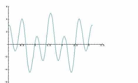
and you should observe a new window containing a plot of these five values plotted against i.5 on the x axis. Any one-dimensional sequence can be plotted in this way; you will find that there are verbs in another script which help you draw, for example, trig series. To draw y= 2sin(5x) + 3cos(12x) from 0 to 2π :

NB. o. means“’ 'pi times' NB. dyadic o. supplies the NB. trig ratios sin,cos,etc

plot x;(2*sin 5*x)+3*cos(12*x)

To print this graph and simultaneously save it as a file, create the following verb :

pg=.dyad define

'res fn'=.x.;y. NB. resolution / filename require'opengl'

glfile fn glsavebmp res

printbmp_jzopengl_ fn

)

Then, with the graph displayed in the plot window, issue the following :

36

500 300 pg 'c:\j406\temp\plot1.bmp'

Graphs can be divided into two categories, those which are essentially algebraic, and those which are inherently geometrical. One example of each is given.

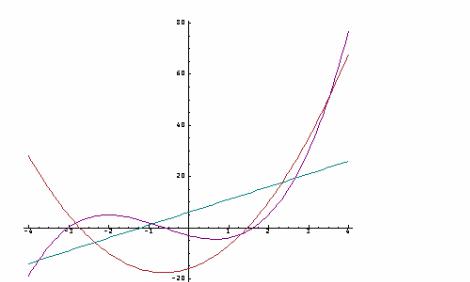
To start with, the polynomial y = 4x2 + 5x – 16 (parabola) is plotted from –4 to 4 by

x=.steps _4 4 100 plot x;_16 5 4 p.x

In order to make the graph a little more interesting the second item in the link is changed into a list of three lists, corresponding to a straight line, a parabola and a cubic respectively :

plot x;((6 5 p.x),:_16 5 4 p.x),_3 _4 2 1 p.x

The example to illustrate geometric graphs involves one possible parametrisation of the curves known as epicycloids and hypocycloids. The first line below illustrates incidentally a technique for making multiple assignments on a single line :

'r R a b'=.2.6 2.36 _40.1 50 x=.(0.01*o.2)*i.101 NB. x from 0 to 2pi p=.(r*cos(a*x))+R*cos(b*x) q=.(r*sin(a*x))+R*sin(b*x)

The command to make the plot is

'labels 0'plot p;q

The left argument of plot is a character string which describes just one of the many possible drawing options, in this case it says “do not display axis labels”.

37

Facilities are also provided which allow the construction of a wide range of drawings. A selection of the basic drawing tools is given below. The graphics window is assumed to be 2 units high and 2 units deep with the origin (0,0) at the centre.

load 'graph'
gdopen''			NB. x	y width height
gdrect _0.4 _0.4 0.8 0.8
gdellipse 0.5 _0.5		0.2 0.4	NB. centre, axis lens.
gdpolygon t=.0.1*7		1 _7 1 7 _4 _2 6 _1 _6 7 1
gdshow''	NB. t is six coordinate			pairs in succession
	NB. window displayed at			this point

The scope for drawing graphics and plots is endless, and ample guidance to all the facilities can be found in the Graph Utilities Lab which is part of the J system.

38

SECTION 9 : RANK

If you have successfully followed the preceding sections, you are now ready to encounter what is one of the most important concepts in J, namely rank.. In section 1 an object called matrix was defined which, although it looked like a matrix, was in fact a list of three four-lists.

3	matrix		0.5
	1	4
_2	3	1	4
0.5	_2	3	1

The fact that it is a list of three lists is made explicit by tally :

#matrix

3

and the fact that each of these three lists is a four-list by shape :

$matrix

3 4

Tallying the shape

#$matrix

2

indicates that matrix is a list of lists, that is after penetrating two list levels primitive objects, in this case numbers, are reached. This can be expressed more concisely by saying that “matrix is an object of rank 2”, and leads to the definition of a verb

rank=.#@$

It is very important to get the order of verbs right in rank since $@# means tally first which always results in a scalar, whose shape is an empty list. An alternative and equivalent definition of rank uses cap which was encountered earlier in section 3 :

rank=.[:#$

The structure involved here is called a capped fork, although a capped hook might be a more appropriate name because the effect is to make the verb pair u v return u v(y) rather than y u v(y) which it would do under the hook rule. In either case :

rank matrix

2

rank c=.3 1 4 0.5 _2

1

rank 7

0

39