

Appendix G.Transformed frequency domain measurements using spice
.pdfAPPENDIX G
Transformed Frequency
Domain Measurements Using
Spice
G.1 INTRODUCTION
Time domain measurements taken on an automatic network analyzer can be easily replicated theoretically for dispersionless transmission lines using the SPICE time domain program simulation. A technique is presented here that gives the type, value, and position of the measured discontinuity directly from time domain measurements. Furthermore the effect of multiple discontinuities can be replicated by SPICE.
Microwave impedance measurements have evolved from the slotted line to the computer-controlled automatic network analyzer. One of the major innovations of the network analyzer made possible by its broadband frequency capability was the simulation of time domain measurements. Though fundamentally a frequency domain machine, the network analyzer has been very useful in doing time domain analysis of broadband circuits. This was demonstrated by the pioneering work of Hines and Stinehelfer [1]. Fundamentally time domain equipment such as the time domain reflectometer have lagged because of the requirement for fast switching devices. However, that has not been true of the software side, as the widespread use of SPICE can readily attest. Here it will be demonstrated how time domain measurements on the network analyzer can be simulated using the transient analysis in SPICE.
There have been several papers that have shown how S parameters can be plotted using SPICE [2,3,4]. SPICE can be used to model physical directional couplers by the interconnection of three transmission lines [5]. By this means, a SPICE model was developed for the characteristics of a network analyzer in the frequency domain. However, the above-mentioned applications are not using the time domain capability of SPICE.
305

306 TRANSFORMED FREQUENCY DOMAIN MEASUREMENTS USING SPICE
First of all, the SPICE S-parameter simulation can be expanded to include unequal input and output impedance levels. This is useful in analyzing impedance steps and transformers with two different resistance levels. Second, rather than using ac steady state voltage sources, a time domain pulse can be used. The automatic network analyzer is made to simulate a time domain reflectometer by mathematically producing an “impulse” that can be replicated in SPICE approximately by using the PULSE function or more accurately by the piecewise linear (PWL) transient function. This SPICE replica of the network analyzer “impulse” can be used to show how various circuit elements react to this “impulse.” Simple formulas are given that can be used to obtain the value of the inductance, capacitance, or impedance step directly from time domain “impulse” data.
G.2 FREQUENCY DOMAIN S-PARAMETERS
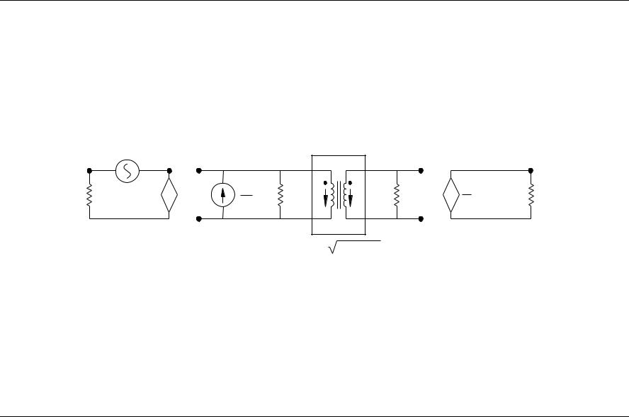
In [4] the S parameters were obtained for a given circuit from SPICE for a twoport circuit in which the input and output resistances were both 50 . However, the conversion circuit used to obtain the S parameters can be modified so that the two ports of the circuit are at different impedance levels (Fig. G.1). This is done by the addition of an ideal transformer whose turns ratio is
n D |
|
|
R01 |
G.1 |
|
|
|
R02 |
|
where R01 and R02 are the characteristic impedance levels of the input and output sides, respectively. The input impedance, Z1, looking into the transformer from the port-1 side is
ZL |
G.2 |
Z1 D n2 |
which is equal to R01 when ZL D R02. The voltage drop caused by the independent current source of value 1/R01 is
1 |
R01jjZ1 D |
Z1 |
G.3 |
|
V1 D |
|
|
||
R01 |
R01 C Z1 |
|||
The voltage at node 11 in Fig. G.1 is numerically the same as S11, since
V 11 |
D |
2V |
|
V |
|
Z1 |
R01 |
G.4 |
|
1 |
in D Z1 |
C R01 |
|||||||
|
|
|
|
||||||
For the output side, the secondary current in the transformer is I2 D I1/n. The portion of current going into the transformer primary from the current source side is
1 |
1 |
1 |
G.5 |
|||
I1 D |
|
R01jjZ1 |
|
D |
|
|
R01 |
Z1 |
Z1 C R01 |
||||
|
|
|
|
Vin=1 |
|
|
|
|
|
|
|
|
|
|
|
|
|
|
|
|
11 |
– |
+ |
10 |
V1 |
|
|
1 : n |
|
|
V |
2 |
|
|
21 |
|
|
|
|
|
|
|
|
|
|
|
|
|
|
|
|
|
|
|
||
|
|
|
|
|
+ |
|
|
|
|
|
|
|
|
|
|
– |
|
|
R |
|
=1 |
|
|
|
1 |
|
|
|
|
|
+ |
2 V |
2 |
R |
|
=1 |
|
|
|
|
2V |
|
R01 I1 |
|
I2 |
ZL |
|
|
|
|||||||
|
11 |
|
|
|
– |
1 |
R01 |
|
|
– n |
|
|
21 |
|
||||
|
|
|
|
|
|
|
|
|
|
|
|
|
|
|
|
+ |
|
|
|
|
|
|
|
|
|
|
n = |
R02 |
/R01 |
|
|
|
|
|
|
|
|
|
|
|
|
|
|
|
|
|
|
|
|
|
|
|
|
|
||
FIGURE G.1 SPICE circuit for finding S parameters with different input and output impedance levels.
307

308 TRANSFORMED FREQUENCY DOMAIN MEASUREMENTS USING SPICE
The voltage at node 2 is
V |
|
I Z |
I1 |
Z |
|
ZL |
G.6 |
|
|
L D Z1 C R01 n |
|||||
|
2 |
D 2 L D n |
|
||||
The voltage across R21 with the marked polarity is V 21 D 2V2/n which, upon replacing V2 with the value above, gives a value for V 21 that is numerically equal to S21:
V 21 D |
2ZL |
D |
2ZL |
D S21 |
G.7 |
Z1 C R01 n2 |
ZL C R02 |
The right-hand side is obtained using Eqs. (G.1) and (G.2). For a matched load when ZL D R02, S21 D 1 as expected. Finding the S22 and S12 for a circuit is achieved by direct analogy. A suggested SPICE listing for finding the S parameters with unequal source and load impedance levels is shown in Section G.6.
G.3 TIME DOMAIN REFLECTOMETRY ANALYSIS
Time domain reflectometer (TDR) measurements from an automatic network analyzer can be directly compared with a theoretical circuit model in the time domain in SPICE. All that is required is to make the two modifications described in Section G.7. Of course, a near-ideal impulse can be implemented in SPICE, but the point of view taken here is to calculate time domain data that would actually be measured using the time domain feature on a network analyzer. Two actual time domain “impulses” were measured on a network analyzer under the conditions in which the maximum frequency was 18 and 26 GHz, respectively. A third “impulse” with a maximum frequency of 50 GHz was calculated from Hewlett Packard’s Microwave Development System (MDS) program. This was justified on the basis that (1) the program and the network analyzer use the same algorithm for the chirp-Z transform and (2) the measured and calculated 18 GHz “impulses” are nearly identical. Circuit responses to “impulses” with different maximum frequency content will of course differ, so the time domain response must be always coupled to the frequencies used in producing the “impulse.”
Two options for representing the network analyzer “impulse” are illustrated in Fig. G.2. The approximate impulse is modeled in SPICE as a PULSE, while the more accurate approach is achieved by using the piecewise linear (PWL) SPICE function. In the present case, the PWL function uses 77 different x, y coordinate pairs to represent the 26 GHz “impulse.” The result is indistinguishable from the measured “impulse” within the resolution of the graph in Fig. G.2. A similar fit was made for the 18 and 50 GHz “impulses.” The piecewise linear fit of the network analyzer “impulses” for use in SPICE are found in Section G.7. The approximate trapezoidal pulse for a 50 source impedance has the advantage of providing results similar to the PWL approximation with a lot less data entry. However, to closely represent the actual time domain response of the network analyzer, the piecewise linear approach should be used.

Pulse Height
|
|
|
|
|
TIME DOMAIN IDENTIFICATION OF CIRCUIT ELEMENTS |
309 |
|||||||||||||||||
1.10 |
|
|
|
|
|
|
|
|
|
|
|
|
|
|
|
|
|
|
|
|
|
|
|
|
|
|
|
|
|
|
|
|
|
|
|
|
|
|
|
|
|
|
|
|
|
|
|
1.00 |
|
|
|
|
|
|
|
|
|
|
|
Approx. Pulse |
|
|
|
|
|
|
|
||||
|
|
|
|
|
|
|
|
|
|
|
|
|
|
|
|
|
|
||||||
0.90 |
|
|
|
|
|
|
|
|
|
|
|
|
|
|
|
|
|
|
|
|
|
|
|
|
|
|
|
|
|
|
|
|
|
|
|
|
|
|
|
|
|
|
|
|
|
|
|
0.80 |
|
|
|
|
|
|
|
|
|
|
|
|
|
|
|
|
|
|
|
|
|
|
|
|
|
|
|
|
|
|
|
|
|
|
|
|
|
|
|
|
|
|
|
|
|
|
|
0.70 |
|
|
|
|
|
|
|
|
|
|
|
|
|
|
|
|
|
|
|
|
|
|
|
|
|
|
|
|
|
|
|
|
|
|
|
|
|
|
|
|
|
|
|
|
|
|
|
0.60 |
|
|
|
|
|
|
|
|
|
|
|
|
|
|
|
|
|
|
|
|
|
|
|
|
|
|
|
|
|
|
|
|
|
|
|
|
|
|
|
|
|
|
|
|
|
|
|
0.50 |
|
|
|
|
|
|
|
|
Measured Pulse |
|
|
|
|
|
|
|
|
|
|||||
|
|
|
|
|
|
|
|
|
|
|
|
|
|
|
|
|
|||||||
0.40 |
|
|
|
|
|
|
|
|
|
|
|
|
|
|
|
|
|
|
|
|
|
|
|
|
|
|
|
|
|
|
|
|
|
|
|
|
|
|
|
|
|
|
|
|
|
|
|
0.30 |
|
|
|
|
|
|
|
|
|
|
|
|
|
|
|
|
|
|
|
|
|
|
|
|
|
|
|
|
|
|
|
|
|
|
|
|
|
|
|
|
|
|
|
|
|
|
|
0.20 |
|
|
|
|
|
|
|
|
|
|
|
|
|
|
|
|
|
|
|
|
|
|
|
|
|
|
|
|
|
|
|
|
|
|
|
|
|
|
|
|
|
|
|
|
|
|
|
0.10 |
|
|
|
|
|
|
|
|
|
|
|
|
|
|
|
|
|
|
|
|
|
|
|
|
|
|
|
|
|
|
|
|
|
|
|
|
|
|
|
|
|
|
|
|
|
|
|
0.00 |
|
|
|
|
|
|
|
|
|
|
|
|
|
|
|
|
|
|
|
|
|
|
|
|
|
|
|
|
|
|
|
|
|
|
|
|
|
|
|
|
|
|
|
|
|
|
|
|
|
10.0 |
20.0 |
30.0 |
40.0 |
50.0 |
60.0 |
70.0 |
80.0 |
90.0 |
100.0 |
||||||||||||
0.0 |
|||||||||||||||||||||||
Time, ps
FIGURE G.2 Measured and approximate trapezoidal 26 GHz pulse used in SPICE analysis.
G.4 TIME DOMAIN IDENTIFICATION OF CIRCUIT ELEMENTS
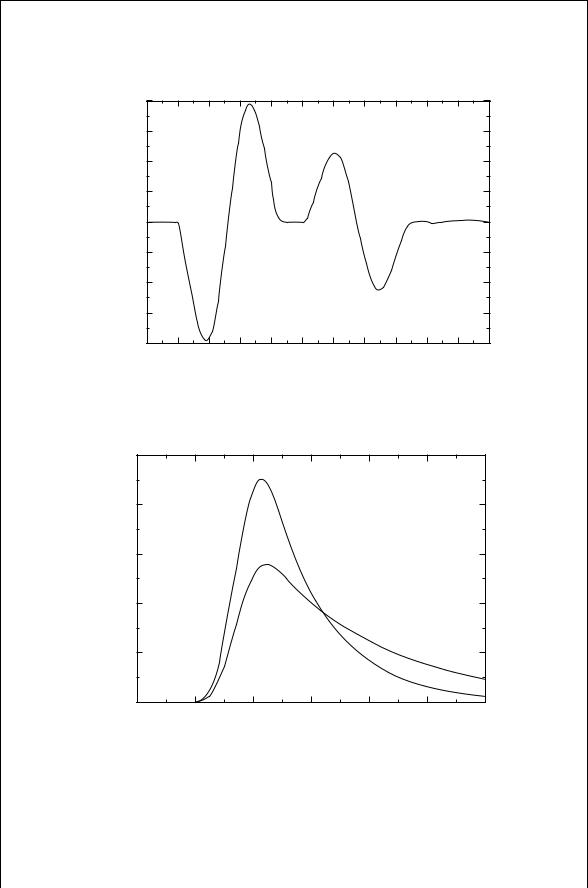
Time domain analysis of discontinuities in broadband circuits enables determining the type of circuit element, the position of the circuit element, and the size of the circuit element causing the discontinuity. For example, if a shunt capacitance is causing the discontinuity, the time domain “impulse” reflection first goes below the baseline, then rises above the baseline and then settles back to the baseline, looking roughly like a single-period sine wave. Figure G.3 shows a typical response to a shunt capacitance and series inductance that are a half wave length apart at 10 GHz. The typical response for a series capacitance is shown in Fig. G.4. A shunt inductance response would look like the negative of the series capacitance. The shunt capacitance, series inductance, series capacitance, shunt inductance, and step in characteristic impedance all have their peculiar time domain signatures.
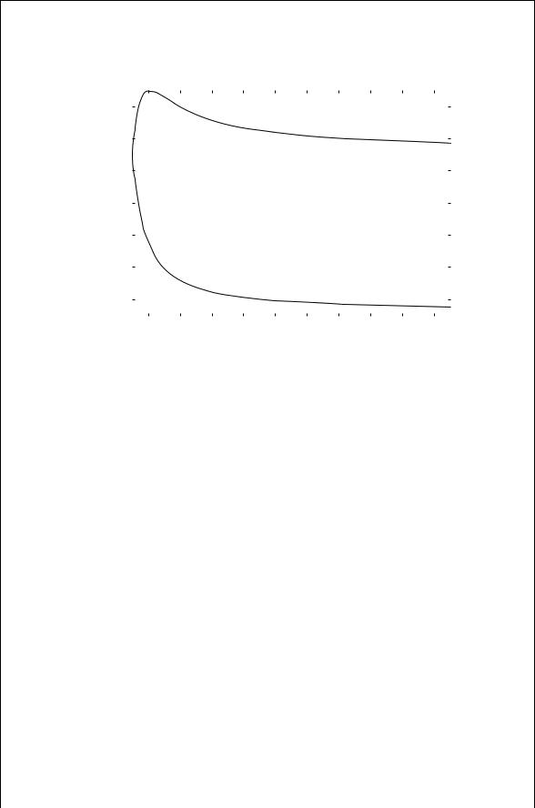
In general, the larger the discontinuity, the larger is the j tj of the time domain response. For the larger shunt capacitances, the magnitude of the dip below the baseline is not equal to the magnitude of the rise above the baseline. So there is some ambiguity in choosing what part of the curve to use to predict the value of the shunt capacitance. A series of capacitance values were tested using both the piecewise linear representation for the network analyzer time domain “impulse.” The results in Fig. G.5 show that if the algebraic maximum of t (the second extremum) is chosen, there are two possible values of capacitance fort. However, the maximum value of the negative excursion of t (the first
310
Γ(t )
TRANSFORMED FREQUENCY DOMAIN MEASUREMENTS USING SPICE
0.100 |
|
|
0.075 |
Series Ind. |
|
|
||
0.050 |
Ind. Max. |
|
Series Cap. |
||
|
||
0.025 |
|
|
0.000 |
|
|
–0.025 |
|
|
–0.050 |
|
|
–0.075 |
Cap. Min. |
|
|
||
–0.100 |
|
75.0 |
100.0 125.0 150.0 175.0 200.0 225.0 250.0 275.0 300.0 325.0 350.0 |
|
Time, ps |
FIGURE G.3 Time domain response from a shunt capacitor separated from a series inductor by a 100 ps 50 transmission line.
0.50 
0.5 pF |
Series Cap. |
0.40
0.30 |
|
1 pF |
|
|
|
|
Γ (t) |
|
|
|
|
|
|
0.20 |
|
|
|
|
|
|
0.10 |
|
|
|
|
|
|
0.00 |
100.0 |
150.0 |
200.0 |
250.0 |
300.0 |
350.0 |
50.0 |
Time, ps
FIGURE G.4 Typical time domain response for a series capacitor.
|
|
|
|
|
TIME DOMAIN IDENTIFICATION OF CIRCUIT ELEMENTS |
311 |
|||||||||||||||||
0.40 |
|
|
|
|
|
|
|
|
|
|
|
|
|
|
|
|
|
|
|
|
|
|
|
|
|
|
|
|
|
|
|
|
|
|
|
|
|
|
|
|
|
|
|
|
|
|
|
0.20 |
|
|
|
|
|
|
|
|
|
|
Max. Γ |
|
|
|
|
|
|
|
|
|
|||
|
|
|
|
|
|
|
|
|
|
|
|
|
|
|
|
|
|
|
|
|
|
|
|
0.00 |
|
|
|
|
|
|
|
|
|
|
|
|
|
|
|
|
|
|
|
|
|
|
|
|
|
|
|
|
|
|
|
|
|
|
|
|
|
|
|
|
|
|
|
|
|
|
|
–0.20 |
|
|
|
|
|
|
|
|
|
|
|
|
|
|
|
|
|
|
|
|
|
|
|
|
|
|
|
|
|
|
|
|
|
|
|
|
|
|
|
|
|
|
|
|
|
|
|
(t ) |
|
|
|
|
|
|
|
|
|
|
|
|
|
|
|
|
|
|
|
|
|
|
|
Γ |
|
|
|
|
|
|
|
|
|
|
|
|
|
|
|
|
|
|
|
|
|
|
|
–0.40 |
|
|
|
|
|
|
|
|
|
|
|
|
|
|
|
|
|
|
|
|
|
|
|
|
|
|
|
|
|
|
|
|
|
|
|
|
|
|
|
|
|
|
|
|
|
|
|
–0.60 |
|
|
|
|
Min. Γ |
|
|
|
|
|
|
|
|
|
|
|
|
|
|
|
|
|
|
|
|
|
|
|
|
|
|
|
|
|
|
|
|
|
|
|
|
|
|
|
|||
|
|
|
|
|
|
|
|
|
|
|
|
|
|
|
|
|
|
|
|
|
|
||
–0.80 |
|
|
|
|
|
|
|
|
|
|
|
|
|
|
|
|
|
|
|
|
|
|
|
|
|
|
|
|
|
|
|
|
|
|
|
|
|
|
|
|
|
|
|
|
|
|
|
–1.00 |
|
|
|
|
|
|
|
|
|
|
|
|
|
|
|
|
|
|
|
|
|
|
|
|
|
|
|
|
|
|
|
|
|
|
|
|
|
|
|
|
|
|
|
|
|
|
|
|
|
2.0 |
4.0 |
6.0 |
8.0 |
10.0 |
12.0 |
14.0 |
16.0 |
18.0 |
20.0 |
||||||||||||
0.0 |
|||||||||||||||||||||||
Capacitance, pF
FIGURE G.5 Maximum and minimum values of the time domain response for a shunt capacitance using the piecewise linear approximation to the measured “impulse.”
extremum) is monotonic, and hence it gives a unique value for the capacitance. The series inductance response is a mirror image to the shunt capacitance about the t D 0 line. Thus the first maximum of t is monotonically related to the value of the series inductance. It is this first maximum of j tj that can be used to find the value of the two types of discontinuities.
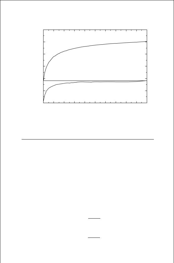
The time domain not only allows determination of the discontinuity type and size but also the discontinuity position in time. Here again there is some ambiguity in the part of the “impulse” response curve that should be used to find the position. For shunt capacitances, a position midway between the lower and upper part of the curve could be used, that is, where t D 0. A comparison of this choice with the theoretical distance is provided in Fig. G.6, where it is seen that this method is accurate if the discontinuity is very small. However, for larger discontinuities a better choice would be at the location of the first extremum of j tj.
The minimum t of the shunt capacitor, the maximum t of the series inductor, the maximum t of the series capacitance, the minimum t of the shunt inductance, and the peak t (either negative or positive) of the impedance step can each be described by a simple formula that could be readily stored in a handheld calculator. These formulas are listed below. The parameters for these expressions are in Table G.1 for the 18 GHz, 26 GHz, and 50 GHz “impulses.”
Shunt capacitance: |
A |
|
|
||
C D |
|
G.8 |
|
||
|
1 C B |
|
312
Time, ps
TRANSFORMED FREQUENCY DOMAIN MEASUREMENTS USING SPICE
180.00
Γ = 0
170.00
160.00
150.00
Actual Position
140.00
130.00Min.Γ
120.00 |
2.0 |
4.0 |
6.0 |
8.0 |
10.0 |
12.0 |
14.0 |
16.0 |
18.0 |
20.0 |
0.0 |
Capacitance, pF
FIGURE G.6 Estimated position (in time) of a shunt capacitor using the minimum value of t and the position where t D 0.
TABLE G.1 Expressions for the Reactance Element Values in Terms of 0
Maximum |
Shunt C, pF |
Series L, nH |
Series C, pF |
Shunt L, nH |
||
Frequency |
CD A/ 1 C B |
L D A/ 1 C B |
CD 1 A / B |
L D 1 A / B |
||
18 |
GHz |
A D 1.212 |
A D 2.965 |
A D 0.9379 |
A D 0.9239 |
|
pulse |
B D 0.9887 |
B D 0.9908 |
B D 1.691 |
B D 0.6892 |
||
26 |
GHz |
A D 0.8216 |
A D 2.061 |
A D 0.9068 |
A D 0.9275 |
|
pulse |
B D 1.004 |
B D 1.010 |
B D 2.624 |
B D 1.036 |
||
50 |
GHz |
A D 0.4275 |
A D 1.091 |
A D 0.9279 |
A D 0.8770 |
|
pulse |
B D 0.9875 |
B D 1.010 |
B D 4.801 |
B D 1.9885 |
|
|
Series inductance: |
|
A |
|
|
L D |
|
G.9 |
||
|
|
|
||
1 |
C |
B |
||
|
|
|
|
|
Series capacitance:
1 A
C D G.10 B
Shunt inductance:
1 A
L D G.11 B

|
|
|
|
MULTIPLE DISCONTINUITIES |
313 |
||
Step in characteristic impedance: |
|
|
|
|
|
|
|
Z0 |
D |
Z |
|
1 C |
|
G.12 |
|
0 1 |
|||||||
0 |
|
|
|||||
Measurements of a given series-mounted chip capacitor on a LCR meter at, say 1 MHz, would not necessarily give accurate correlation with a time domain model of a simple series capacitance as modeled by Eq. (G.10) or direct measurements on a network analyzer. However, a better fit with the time domain data can be obtained by using a model of a high-frequency capacitor as described in Chapter 2.
G.5 MULTIPLE DISCONTINUITIES
The formulas above are correct when there is only one significant discontinuity in the circuit that is being measured. When there are multiple discontinuities, the SPICE analysis will also display the results that would be expected in a real time domain reflectometer measurement. The gating error in measuring a discontinuity in the presence of other discontinuities is analyzed in [6]. That analysis uses a rectangular gating function with a depth of 40 dB rather than the chirp-Z transform in the network analyzer software. Four sources of error are identified. The first is out-of-gate attenuation associated with incomplete suppression of reflections outside the gating function. The second is truncation error where the gate is made too narrow to pick up all of the response due to the discontinuity in question. The third is masking error where the transmission coefficients of previous discontinuities reduces the signal getting to the discontinuity under investigation. The fourth is multi-reflection aliasing error that occurs when the circuit has commensurate line lengths, and the residual reflection of one discontinuity adds to or subtracts from the reflection of the discontinuity under investigation.
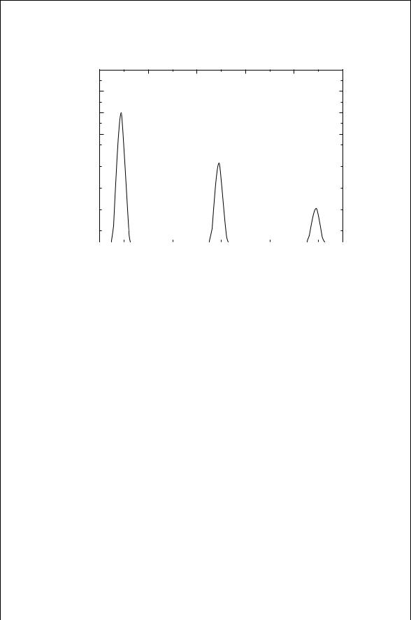
When two discontinuities are sufficiently separated in time, each can be analyzed separately, though the accuracy of predicting the later discontinuities from the formulas in Table G.1 are less accurate than when there is only one discontinuity. Three impedance steps are set up such that if they were alone, they would have had a t of 0.3, 0.2, and 0.1, respectively (Fig. G.7), as is done by [6]. However, when the three steps are put in one circuit suitably separated from one another, the SPICE analysis shows that t D 0.3 (0% error), t D 0.181 (9.6% error), and t D 0.087 to 0.076 (12.9% to 24% error depending on whether line lengths are commensurate). The estimated errors in [6] are 0%, 12%, and 20%, respectively, which correlate well with the SPICE results given the approximations that are employed.
In addition the technique described here can be used in a wide variety of circuits to model two elements that are too close together to be resolved separately in time. Adjustment of a theoretical time domain model to make its response match that of the measured time domain measurements gives a method to extract an equivalent circuit in the time domain.
314
Γ (t )
TRANSFORMED FREQUENCY DOMAIN MEASUREMENTS USING SPICE
0.40
0.35
0.30 0.3
0.25
0.20 |
|
|
|
|
|
|
0.181 |
|
|
|
|
|
|
|
|
|
|
|
|
|
|
|
|
|
|||
0.15 |
|
|
|
|
|
|
|
|
|
|
|
|
|
|
|
|
|
|
|
|
|
|
|
|
|
|
|
0.10 |
|
|
|
|
|
|
|
|
|
|
0.076 |
|
|
|
|
|
|
|
|
|
|
|
|
|
|
||
0.05 |
|
|
|
|
|
|
|
|
|
|
|
|
|
|
|
|
|
|
|
|
|
|
|
|
|
|
|
0.00 |
|
|
|
|
|
|
|
|
|
|
|
|
|
|
|
|
|
|
|
|
|
|
|
|
|
|
|
|
|
0.2 |
0.4 |
0.6 |
0.8 |
1.0 |
|||||||
0.0 |
|||||||||||||
Time, ns
FIGURE G.7 Predicted response from three discontinuities whose actual reflection coefficients are 0.3, 0.2, and 0.1.
G.6 SAMPLE SPICE LIST
The SPICE listing below can be used to find the S11 D V11 and S21 D V21 parameters when the source and load resistances are 50 , and the circuit is
terminated with a 50 load. These may be changed in the PARAM statement. The circuit to be analyzed is entered in the SUBCKT section. The number of frequencies and the frequency range must also be added to the ac statement. The following net list was used in PSPICE. Other versions of SPICE may require some minor modifications as noted in the net list.
Analysis of a circuit for S11 and S21
*
*R01 and R02 are input and output resistance levels.
*RL is the load resistance. The load may be supplemented
*with additional elements.
.PARAM R01=50, R02=50. RLOAD=50. IIN=-1/R01
.FUNC |
N(R01,R02) SQRT(R02/R01) |
||||
R01 |
1 |
0 |
R01 |
|
|
VIN |
10 |
11 |
AC |
1 |
|
GI1 |
1 |
0 |
VALUE=-V(10,11)/R01 |
||
*GI1 |
1 |
0 |
10 |
11 |
”-1/R01” |
E11 |
10 |
0 |
1 |
0 |
2 |
R11 |
11 |
0 |
1 |
|
|