Bandara G.E.Intelligent fuzzy controller for a lead acid battery charger

INTELLIGENT FUZZY CONTROLLER FOR A LEAD ACID

BATTERY CHARGER

G.E.M.D.C.Bandara*, Ratcho M. Ivanov and Stoyan Gishin

Department of Electronics Engineering, Faculty of Electronics

Sofia 1000, Bulgaria

Phone: [phone], Fax: [phone]

Email*:[e-mail]

ABSTRACT: During the last ten years, fuzzy Control has emerged as the most popular method in non-linear process control, due to the simplicity of implementation, robustness and independence from mathematical presentation of the control system. Fuzzy control can be applied to almost every control system, where mathematical model is not available or difficult to derive from existing data of the system.

Fuzzy control of a Lead-Acid Battery Charger is being investigated in this paper. Effective control of the charging process is complex due to the exponential relationship between the charging current and the charging time. Classical control algorithms such as PID, PI etc., are difficult to implement in this event, due to the unavailability of the value for the coefficient of discharge in the exponential current-time relationship and switching over of the control inputs during the two phases of the charging process.

Initial peak charging current is reduced stepwise during the charging time and the quantity of the energy necessary for the charging process is effectively reduced. An intelligent Microcontroller based digital architecture is developed to sense the charging current and the present charge, after which fast fuzzy inference mechanism defines the next level of the charging current. Delay time of the switching of the main supply is calculated after the fuzzy inference, and the power switch is switched accordingly.

Experimental results and expert knowledge are used for tuning of the membership functions and the rule base of the fuzzy controller.

Keywords: Fuzzy sets, fuzzy control, fuzzification, membership functions, regulator, fuzzy inference, defuzzification, centre of gravity, microcontroller

INTRODUCTION

Rechargeable batteries have wide variety of applications not only in the automobile industry but also in telecommunications, energy industry, medicine, defence applications and almost every where in industrial applications, where continuos operating power is required. Methods used for charging such batteries vary depending on their chemical composition, capacity, and methods of the construction and the type of the exploitation. Efficiency of the charging algorithms are also depend on the amount of current used for the charging process, levels of the oscillations in the charging current, charging voltage levels, charging time and the fluctuations in the temperature during the charging process.

In this paper design of an intelligent universal battery charger, in which the control algorithm is implemented with fuzzy logic is discussed. The intelligent digital architecture is implemented with Motorola's latest 16bit microcontroller MC68HC812A4, which comes with a number of instructions specialised for fuzzy logic programming (Bandara, 1997). Microcontroller's light integration module has almost all necessary peripherals to design this controller, but an external analogue to digital converter is used for measuring the current and the voltage to achieve high resolution. Implementing one of the very effective and latest charging algorithms with fuzzy logic is discussed in detail. The fuzzy control algorithm achieves the charging task in two phases. During the first phase the voltage is maintained below a maximum level given by the operator during the initial setting up process which is done in dialogue mode and the current is regulated to the set maximum level. Set point of the current is closely related with the capacity of the battery and this is taken in to mind when writing the program. The second phase starts when the battery voltage reaches a specific value

depending again on the capacity and number of cells available in the battery. During this phase control variable switches over from current to voltage and the voltage is maintained at a given by the operator level, while the current is gradually decreasing until it reaches a value set in the program depending on the capacity of the battery. A Lead-Acid battery is used during the experiments, but the device can also be connected to other types of rechargeable batteries such as Ni-Cd.

FUNDAMENTAL CONCEPTS OF EXPLOITATION AND CHARGING OF BATTERIES

There are two basic modes of exploitation of the batteries (Teoharov, 1995):

1.Continuos mode of exploitation

2.Standby or floating mode of exploitation.

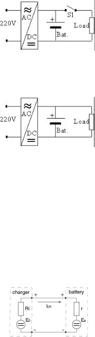
Figure 1: Continuos mode of operation

In the first mode (Fig.1), the battery is connected to the charging device only after falling to provide the required energy as a result of discharging the battery to a large extent due to a long period of exploitation. The battery is disconnected from the load during the charging process and it consumes energy from the charging device. The battery is connected to the charging device and the load simultaneously during the second mode of operation (Fig. 2).

Figure 2: Stand-by mode of operation

The charging device has two distinctive types of functions during this mode of operation. First, the charging device functions as a current generator, immediately after the discharging of the battery. The high initial current is characteristic for this mode and it secures quick charging of the battery at the beginning of the charging cycle, where 80% - 90% of the capacity is charged. The charging device moves onto the second phase when the voltage reaches the required value. The charging device has the function of a voltage generator at the second phase and the fixed voltage, which was achieved at the first stage, is continuously maintained. The battery consumes only an amount of current that is required for the charging process. Therefore the current gradually decreases and stabilises at a value which is called "current of the under charge". This low current compensates self-charging current of the battery.

METHODS FOR CHARGING THE BATTERIES

The charging devices of batteries function in a specific mode where the load has a capacitive character and can be considered as an infinite capacitor, which has the equivalent circuit shown in the Figure 3.

Figure 3: Equivalent circuit of a charging process

The internal resistance of the battery is defined as 0.25/ Q per battery cell, (Teoharov, 1995) where Q is the capacity of the battery. As an example, let's consider a 12V battery, consisting of six cells and has the capacity of 120Ah. Internal resistance of this battery can be calculated as follows:

0.25 / 120 = 0.00208 x 6 = 0.0125 Ω

If the charging device is assumed to have fluctuations of the output voltage at levels of 600mV - 800mV, the coefficient of the fluctuations becomes 9.6% and the pulsating charge current has the following value:

0.8 / 0.0125 = 64A

This pulse can destroy the battery if it is not maintained below the required level. This example shows us that the level of fluctuations of the charging current must be limited in order to avoid heating and boiling of the acids in the composition and to increase the durability of the battery.

There are a number of methods for charging the batteries (Teoharov, 1995).

1.Charging with constant current

2.Charging with a semi-constant current

3.Charging with constant voltage

4.Multistage charging according to the Ampere - Hour rule and two stage charging cycle which simplifies the multistage charging method, where the charging cycle at first with a constant current and next with constant voltage.

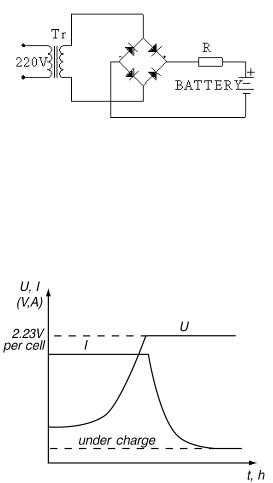
The first method is rarely used in general application, but is very effective when charging a large number of serially connected batteries. This method has a small coefficient of efficiency and adversely effect over the characteristics of the battery and the durability, while the second method has very simple architecture consisting of a transformer, rectifier bridge and a current limiting resistor as shown in Figure 4.

Figure 4: Charging with a semi-constant current

This method is also called as "Taper charging" and it is also not recommendable due to constant current characteristics of the charging device adversely effect especially the Lead - acid batteries. Batteries are normally overcharged due to the very high current and reduce life of the batteries. This method also characterises a low coefficient of efficiency due to the resistor and initial current limitation is required. In the third method (Fig. 5) initial charging current is very high, but is maintained below a certain level (10% -25% of the capacity of the battery) to protect the battery. The current gradually decreases towards the end of the charging cycle. Charging voltage must be set depending on the capacity of the battery and it's temperature characteristics.

Figure 5: Charging with a constant voltage

The forth method is widely accepted as the best and is discussed below in detail.

This method is recommended to charging the Lead - acid batteries with in a short time and maintains the battery in standby mode.

AMPHERE-HOUR RULE (Ah RULE)

It is important to mention the Ampere - hour rule here. It states that at any moment of the charging cycle the charging current expressed in amperes must not exceed the capacity of the battery at that moment, expressed in Ampere-hours.

This rule mathematically expresses the charging current with the following formula:

I	ch	= C . e−t	→ (1)
		disch

Where, Ich - charging current in amperes, Cdisch - capacity discharged from the battery, t - charging time. Figure.6 (Balogh, 1998) shows some charging curves of an n umber of Lead - acid batteries.

Figure 6: Exponential charging curves of Lead - acid batteries

The above curves are derived by assuming that the batteries are completely discharged. By integrating both sides and multiplying by dt the equation (1) can be expressed as follows:

òIch .dt = Cdish òe− t .dt

The left-hand side of the expressions represents the capacity of the battery during the charging cycle. Therefore,

Cbat = Cdisch òe−t .dt = −Cdisch e−t + c

Where, c - constant of integration which can be found from the initial conditions: t = 0, Cbat = 0; hence c = Cdisch ; therefore Cch can be expressed by the following expression:

C	= C	(1 − e− t ) → (2)
Bat	disch

Table 1 shows the importance of the Ampere - hour rule when charging the Lead - acid batteries. Experimentally obtained percentages shown in the table is the percentage of the charge from the total capacity of the battery, when charged according to the above-mentioned rule.

t, h	0	0.5	1.0	2.0	3.0	5.0
Cbat %	0	39.2	63.1	87.5	95.0	99.4

Table 1: Change of the capacity of the battery during the charging cycle in Ah.

Application of the Ampere - hour rule for charging the Lead - acid batteries can be considered as the most efficient method, when considering the time and the energy saved by this method. Implementation of this method is briefly shown in figure 7.

Figure 7: Current and Voltage curves for a charging cycle of a Lead - acid battery according to the Ampere-hour rule

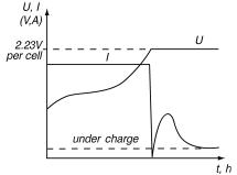
The charging technique given in figure 7 can easily be simplified into a two stage charging cycle, where the charging time can be reduced to almost 50% and thus the energy required to charge the battery, while keeping all the advantages of the method. This shorter and efficient implementation of the ampere - hour rule is tested in the fuzzy algorithm and the highest performance achieved in the practical implementation is once again proved. Figure.8 shows characteristics of such charging device. During the first phase the charging current is controlled to a certain value and the voltage of the battery gradually increases, but kept below a certain maximum level which is defined according to the characteristics of the battery. The device moves onto the second phase when the voltage reaches to a certain level which is defined by the characteristics of the battery and normally this is taken as 90% of the total capacity of the battery.

Figure 8: Simplified Ampere - hour charging method

The voltage of the battery must be regulated at a value which is smaller than the value at which the second phase started and the current gradually decreases, because the battery has charged up to 90% of it's capacity during the first phase of the charging cycle. Moving into the second stage also protects the battery from over charging. The output values must be in the following limits in this mode (Table 2):

Initial charging current	(10% - 25%)A of the capacity of the battery
Charging voltage
First phase	2.45 V per cell ( 2.5 V per cell maximum)
Second phase	2.28 V per cell ( 2.3V per cell maximum)
Undercharge current at the end of	(0.4% - 0.5 % )A of the capacity of the battery
the second phase
Temperature compensation
Stand-by mode	3mV / °C per cell
Continuos mode	4mV / °C per cell

Table 2: Initial settings for the simplified ampere - hour charging method

FUNDAMENTALES OF FUZZY CONTROL

Fuzzy logic and fundamental concepts of fuzzy control was first introduced by Lotfi Zadeh (Zadeh, 1973) and successfully applied (Mamdani, 1974) in 1970's in an attempt to provide an easy way to control non-linear processes, for which mathematical model is difficult to derive. Since then fuzzy logic and fuzzy control became more popular and many applications to industrial processes have been published (Mattavelli, 1997)

Fuzzy logic's distinctive feature is the use of linguistic variables instead the numerical variables. These are defined as sentences in a natural language (such as current is low, voltage is medium) and can be represented by fuzzy sets.

FUZZY SETS AND MEMBERSHIP FUNCTIONS (ZADEH, 1973)

Definition:

If X is a collection of objects denoted generically by x then a fuzzy set A in X is a set of ordered pairs:

A = {(x, μ A (x)), x X }

Where μA(x) is called the membership function or grade of membership of x in A, and has the values between 0 and 1,

μ A : X → [0,1] . The range of the membership function is the subset of the non-negative real numbers whose supremum is finite. When representing the degree of membership, elements with zero degree of membership are not listed. In the above definition the X is defined as universe of discourse and is defined in a specific problem. The membership functions can have various forms triangular, trapezoidal, singleton etc. Singleton representation of the membership functions is a special form where the fuzzy set A is described by only one element x0 with μA(x0) =1,

while all of the other elements have a membership grade of zero.

FUZZY CONTROL

Every fuzzy controller has three basic steps. Fuzzification, rules evaluation and defuzzification. Architecture of a fuzzy logic control system is shown in Fig. 9.

Figure 9: Fuzzy Logic control system architecture

The application concerned here is a two input one output fuzzy system; therefore design of an inference engine for such a controller is discussed in detail.

MEMBERSHIP FUNCTION DATABASE DESIGN

Both inputs of the controller are taken as the error (ε k ) and the change of the error ( ε k ) , which can be calculated as follows:

Error(ε k ) = Setpo int k − Outputk

Where k is the kth sample time.

Change of Error( ε k )= ε k − ε k −1

Lets consider the fuzzy set A in the universe of discourse X. The fuzzy set A can be represented as a set of ordered pairs of a generic element x and its grade of membership function A = μ (x) / x . When X is continuos, the fuzzy set A can

be written as	A = ò	μ ( x)/ x
	X	, where the integral sign is used to represent the union of the fuzzy singletons. First the

control variables must be divided into a set of fuzzy regions, which are given unique names called labels, within the domain of the variables. In our case labels: positive big (PB), positive medium (PM), positive small (PS), Zero (Z),

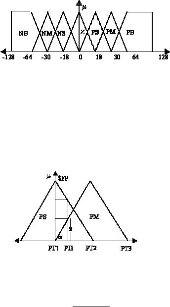
negative small (NS), negative medium (NM) and negative big (NB) are used. Each of these sets is defined by the left and right limits of the set. The fuzziness of each label is calculated during the fuzzification step. The universe of discourse in our case is the minimum and maximum values of the analogue to digital converter, therefore the universe of discourse for the problem discussed is (-128, +127). The fuzzy sets for the voltage error variable is shown in fig.10.

Figure 10: Membership functions for the input variables

FUZZIFICATION

In fuzzy logic controller’s resolution of the system depends on the fuzziness of the control variables, whereas the fuzziness of the control variables depends on the fuzziness of their membership functions. In the fuzzification (Bandara, 1997) phase actual measured input values are mapped into fuzzy membership functions. Every actual value falls in two membership functions, as an example let's assume that the variable error = 23 (PTi) in hexadecimal code.

One membership value is calculated using the similar triangle principle, while the other is calculated from orthogonality of the membership function triangles.

Figure 11: Calculation of fuzziness of input variables

According to Figure. 11, fuzziness of the input variable Error = $23 in the membership function PM can be calculated as follows:

( PTi − PT1 ) x = FF × ( PT2 − PT1 )

Here x gets a value in hexadecimal code and fuzziness of this input value in the membership function PS equals to $FF-x according to the orthogonal principle.

RULE EVALUATION AND THE RULE BASE DESIGN

Rule evaluation is the central element of a fuzzy logic control system. This step processes a list of rules from the knowledge base using current fuzzy input values from RAM to produce a list of fuzzy outputs in RAM. These fuzzy outputs can be taught as raw suggestions for what the systems output should be in response to the current input conditions.

The design of fuzzy control rules (Togai, 1985) involves writing rules that relate the input variables to the output model properties. These rules are expressed as IF - THEN statements and the syntax is as follows:

If {error (ε) is X and change of error (Δε) is Y} then {control output is Z}

The first part of the rule is called antecedents and the second part is called consequent. Such a group of rules forms the fuzzy rule base. Although there isn't an well-organised theoretical foundation to define the rule base, there are a number of methods to derive the rule base. State space method (Lee, 1990), application of expert knowledge to define the rule base (Mamdani, 1974), fuzzy modelling of the process by using fuzzy implications, concerns with inputs, state variables and outputs (Togai, 1985), self organising control based on meta-rules from which control rules can be created or changed (Tong, 1980) and modelling operators controller actions (Togai, 1985).

In the application discussed here state space method (Lee, 1990) is preferred for determining the rules due to it's close relation with the system's transfer function. The rule base for the control systems is shown in Fig. 12.

Figure 12: Rule base of the controller

The Min - Max method (Lee, 1990) was used in the rule evaluation process. In Min - Max rule evaluation antecedents are connected with the Min operation and the result is max'ed with the consequents.

DEFUZZIFICATION

The final step in the fuzzy logic controller is to combine the fuzzy output into a crisp systems output. The output membership functions in the control system are represented by singletons. Output of the battery charger is the delay time in which the triac doesn't pass through the sinusoidal waveform, therefore the universe of discourse has the values (-1792, +1792), which stands for the change of output within a range of (-2V, +2V). The output membership functions of the systems are shown in Figure 13.

Figure 13: Output membership functions

There are various methods to calculate the crisp output of the system (Lee, 1990). Centre of Gravity (COG) method is used in our application due to better results it gives. The COG for our application, is expressed mathematically in the following equation:

7

åSi × Fi

t = 1

7

åFi

1

Where Si - ith singleton position, Fi - Fuzziness of the ith singleton and the t is the change of the present system delay in μS, and this number represents a signed number which is added or subtracted from the present delay to generate the next system response.

EXPERIMENTAL SET-UP

A lead acid battery with 44Ah capacity is used in the experiments. The evaluation board for MC68HC812A4 developed by the authors (Bandara, 1998) is used with some other circuits as shown in Figure 14.

Figure 14: Detailed block diagram of the controller

EXPERIMENTAL RESULTS AND DISCUSSION OF THE PERFORMANCE.

A fuzzy controller for a lead-acid battery charger is developed. At the first stage of the charging cycle the control input variable becomes the current and only the voltage is measured and kept below the maximum level. At the next stage the input variable becomes the voltage and the current is monitored. Specific Fuzzy logic instructions in the HC12 are used to build the fuzzy regulator and its performance was proved to be very high. This regulator takes only 3mS to generate the next system input. Volt–Ampere characteristics of the controller are shown in Figure 15.

Figure 15: Change of voltage during the charging cycle

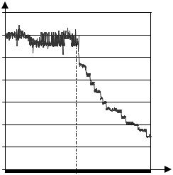
High response time and the extremely low overshoot time were a result of fine-tuning of the fuzzy regulator with the help of an expert. Change of the current during the charging cycle is shown in Figure 16. Switching over of the regulators is taken place at the point A. Figures 15 and 16 show that this switching is smooth and the effect on the working point of the system is minimal.

	7
	6					Setpoint = 6A
	5
I(A	4
	3
	2
	1
	0					A
		109	217	325	433	541	649	757	865	973
	1										time,s

Figure 16: Change of current during the charging cycle

Controller's performance was slightly poor when only 19 rules were used, therefore finally we moved onto the full rule list.

CONCLUSION

High performance and very effective battery charger is developed. All critical set points are completely independent from hardware, which guarantees precise control. Data logging and the virtual instrument created in Lab View showed surprisingly low standard deviation for both regulators. The standard deviations for the voltage regulator was as low as 0.01% and for the current regulator it was recorded as 0.1%. User friendly software developed for this purpose provides an easy way to input the initial data including the charging current and the voltage at which the second phase begins. Charging time in this method is reduced to almost 50% in comparison to the classical methods. For a fully discharged battery required charging time was approximately 3 hours. The energy saved by method is also a good reason for implementing the method in industrial environments. This method also prevents the battery from over charging as a result of the very well tuned fuzzy regulator. Small overshoots and undershoots of the current regulator are the only points which need further tuning of the membership functions for this regulator. But, approximately 0.2% accuracy is achieved in the current regulator too.

FUTURE STUDIES

Fluctuations in the temperature during the charging cycle was neglected when designing the regulator, but for highest performance the changes in the temperature must be taken into account and the regulator must be modified accordingly. The current regulator needs some fine-tuning of the membership functions, possibly by genetic algorithms or neural network based methods. The power electronics section of the design can be replaced with a switching regulator, which simplifies the device.