BookBody

Sec. 6.7] Definite Clause grammars 141

semicolon (and then a RETURN). In the last case, the Prolog system will search for another instantiation of X.

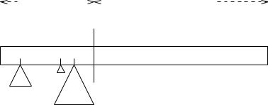
Not every fact is as simple as the one in the example above. For instance, a Prolog clause that could tell us something about antique furniture is the following:

antique_furniture(Obj, Age) :- furniture(Obj), Age>100.

Here we see a conjunction of two goals: an object Obj with age Age is an antique piece of furniture if it is a piece of furniture AND its age is more than a 100 years.

An important data structure in Prolog is the list. The empty list is denoted by [],

[a]is a list with head a and tail [], [a,b,c] is a list with head a and tail [b,c]. Many Prolog systems allow us to specify grammars. For instance, the grammar of

Figure 6.6, looks like the one in Figure 6.14, when written in Prolog. The terminal symbols appear as lists of one element.

% Our example grammar in Definite Clause Grammar format.

sn --> dn, cn. sn --> an, bn. an --> [a].

an --> [a], an. bn --> [b], [c].

bn --> [b], bn, [c]. cn --> [c].

cn --> [c], cn. dn --> [a], [b].

dn --> [a], dn, [b].

Figure 6.14 An example grammar in Prolog

The Prolog system translates these rules into Prolog clauses, also sometimes called definite clauses, which we can investigate with the listing question:

| ?- listing(dn).

dn(_3,_4) :- c(_3,a,_13), c(_13,b,_4).

dn(_3,_4) :- c(_3,a,_13), dn(_13,_14), c(_14,b,_4).

yes

| ?- listing(sn).

sn(_3,_4) :-

142

General directional top-down methods

[Ch. 6

dn(_3,_13), cn(_13,_4).

sn(_3,_4) :- an(_3,_13), bn(_13,_4).

yes

We see that the clauses for the non-terminals have two parameter variables. The first one represents the part of the sentence that has yet to be parsed, and the second one represents the tail end of the first one, being the part that is not covered by the current invocation of this non-terminal.

The built-in c-clause matches the head of its first parameter with the second parameter, and the tail of this parameter with the third parameter. A sample Prolog session with this grammar is presented below:

& prolog

C-Prolog version 1.5 | ?- [gram1].

gram1 consulted 968 bytes .133333 sec.

yes

We have now started the Prolog system, and requested it to consult the file containing the grammar. Here, the grammar resides in a file called gram1.

| ?- sn(A,[]).

A = [a,b,c] ;

A = [a,b,c,c] ;

A = [a,b,c,c,c] .

yes

We have now asked the system to generate some sentences, by passing an uninstantiated variable to sn, and requesting the system to find other instantiations twice. The Prolog system uses a depth-first searching mechanism, which is not suitable for sentence generation. It will only generate sentences starting with an a, followed by a b, and then followed by an ever increasing number of c’s.

| ?- sn([a,b,c],[]).

yes

| ?- sn([a,a,b,c],[]).

yes

Sec. 6.7]

Definite Clause grammars

143

| ?- sn([a,b,c,c],[]).

yes

| ?- sn([a,a,a,b,b,c,c,c],[]).

no

| ?- halt.

[ Prolog execution halted ]

&

Here we have asked the system to recognize some sentences, including two on which the naive backtracking parser of Section 6.6.1 failed: aabc and abcc. This session demonstrates that we can use Definite Clause Grammars for recognizing sentences, and to a lesser extent also for generating sentences.

Cohen and Hickey [CF 1987] discuss this and other applications of Prolog in parsers in more detail. For more information on Prolog, see Programming in Prolog by William F. Clocksin and Christopher S. Mellish (Springer-Verlag, Berlin, 1981).

7

General bottom-up parsing

As explained in Section 3.3.2, bottom-up parsing is conceptually very simple. At all times we are in the possession of a sentential form that derives from the input text through a series of left-most reductions (which mirrored right-most productions). There is a cut somewhere in this sentential form which separates the already reduced part (on the left) from the yet unexamined part (on the right). See Figure 7.1. The part on the left is called the “stack” and the part on the right “rest of input”. The latter contains terminal symbols only, since it is an unprocessed part of the original sentence, while the stack contains a mixture of terminals and non-terminals, resulting from recognized right-hand sides. We can complete the picture by keeping the partial parse trees created by the reductions attached to their non-terminals. Now all the terminal symbols of the original input are still there; the terminals in the stack are one part of them, another part is semi-hidden in the partial parse trees and the rest is untouched in the rest of the input. No information is lost, but some structure has been added. When the bottom-up parser has reached the situation where the rest of the input is empty and the stack contains only the start symbol, we have achieved a parsing and the parse tree will be dangling from the start symbol. This view clearly exposes the idea that parsing is nothing but structuring the input.

STACK

REST OF INPUT

terminals

CUT

terminals

and

only

non-terminals

tg Nf te td Nc Nb ta t1 t2 t3 . .

partial parse trees

Figure 7.1 The structure of a bottom-up parse

The cut between stack and rest of input is often drawn as a gap, for clarity and since in actual implementations the two are often represented quite differently in the

Ch. 7]

General bottom-up parsing

145

parser.

tg Nf te td Nc Nb ta

.

.

.

t

N

f

t

t

N

c

N

b

t

.. t

g

e

d

a. 1

.

	.
	.
t	.	t . .
	.. t
1	. 2	3
	.

shifting t1

t2 t3 . .

Figure 7.2 A shift move in a bottom-up automaton

.

.

.

t

N

f

t

t

.. N

c

N

b

t

g

e

d.

a

.

t1 t2 t3 . .

reducing NcNbta to R

				.
				.
				.						t t t . .
t N		t t .. R
g		f e			d.					1 2 3
				.
			. . . . . . . . . . . . .
.									.
.									.
..				N			N	t ..
.						c		b	a .
. . .						. . . . . . . . . .

Figure 7.3 A reduce move in a bottom-up automaton

Our non-deterministic bottom-up automaton can make only two moves: shift and reduce; see Figures 7.2 and 7.3. During a shift, a (terminal) symbol is shifted from the rest of input to the stack; t1 is shifted in Figure 7.2. During a reduce move, a number of symbols from the right end of the stack, which form the right-hand side of a rule for a non-terminal, are replaced by that non-terminal and are attached to that non-terminal as the partial parse tree. NcNbta is reduced to R in Figure 7.3; note that the original NcNbta are still present inside the partial parse tree. There would, in principle, be no harm in performing the instructions backwards, an unshift and unreduce, although they would seem to move us away from our goal, which is to obtain a parse tree. We shall see that we need them to do backtracking.

At any point in time the machine can either shift (if there is an input symbol left) or not, or it can do one or more reductions, depending on how many right-hand sides can be recognized. If it cannot do either, it will have to resort to the backtrack moves,

146

General bottom-up parsing

[Ch. 7

to find other possibilities. And if it cannot even do that, it is finished, and has found all (zero or more) parsings.

7.1 PARSING BY SEARCHING

The only problem left is how to guide the automaton through all of the possibilities. This is easily recognized as a search problem, which can be handled by a depth-first or a breadth-first method. We shall now see how the machinery operates for both search methods. Since the effects are exponential in size, even the smallest example gets quite big and we shall use the unrealistic grammar of Figure 7.4. The test input is aaaab.

1.	SS	->	a	S	b
2.	S	->	S	a	b

3.S -> a a a

Figure 7.4 A simple grammar for demonstration purposes

(a)	éaaaab		(k)	aSbù		(s)	Sabù
(b)	a éaaab			aa3a			aaa
(c)	aa éaab		(l)	aSù b		(t)	Saù b
				aa3a			aaa
(d)	aaa3 éab		(m)	aaa3aù b		(u)	Sù ab
(e)	aaa3a3 éb		(n)	aaa3ù ab			aaa
(f)	aaa3a3bù		(o)	S éab		(v)	aaaù ab
(g)	aaa3a3ù b			aaa		(w)	aaù aab
(h)	aS éb		(p)	Sa éb		(x)	aù aaab
	aa3a			aaa		(y)	ù aaaab
(i)	aSb1ù		(q)	Sab2ù
	aa3a			aaa
(j)	Sù		(r)	Sù
	aSb			Sab
	aa3a		aaa

Figure 7.5 Stages for the depth-first parsing of aaaab

7.1.1 Depth-first (backtracking) parsing

Refer to Figure 7.5, where the gap for a shift is shown as é and that for an unshift as ù . At first the gap is to the left of the entire input (a) and shifting is the only alternative; likewise with (b) and (c). In (d) we have a choice, either to shift, or to reduce using rule 3; we shift, but remember the possible reduction(s); the rule numbers of these are

Sec. 7.1]

Parsing by searching

147

shown as subscripts to the symbols in the stack. Idem in (e). In (f) we have reached a position in which shift fails, reduce fails (there are no right-hand sides aaaab, aaab, aab, ab or b) and there are no stored alternatives. So we start backtracking by unshifting (g). Here we find a stored alternative, “reduce by 3”, which we apply (h), deleting the index for the stored alternative in the process; now we can shift again (i). No more shifts are possible, but a reduce by 1 gives us a parsing (j). After having enjoyed our success we unreduce (k); note that (k) only differs from (i) in that the stored alternative 1 has been consumed. Unshifting, unreducing and again unshifting brings us to (n) where we find a stored alternative, “reduce by 3”. After reducing (o) we can shift again, twice (p, q). A “reduce by 2” produces the second parsing (r). The rest of the road is barren: unreduce, unshift, unshift, unreduce (v) and three unshifts bring the automaton to a halt, with the input reconstructed (y).

(a1)		initial	(f1)	aaaab	shifted from e1
(b1)	a	shifted from a1	(f2)	Sab	shifted from e2
(c1)	aa	shifted from b1		aaa
(d1)	aaa	shifted from c1	(f3)	aSb	shifted from e3
				aaa
(d2)	S	reduced from d1	(f4)	S	reduced from f2
	aaa
				Sab
(e1)	aaaa	shifted from d1		aaa
(e2)	Sa	shifted from d2	(f5)	S	reduced from f3
	aaa			aSb
(e3)	aS	reduced from e1		aaa

aaa

Figure 7.6 Stages for the breadth-first parsing of aaaab

7.1.2 Breadth-first (on-line) parsing

Breadth-first bottom-up parsing is simpler than depth-first, at the expense of a far larger memory requirement. Since the input symbols will be brought in one by one (each causing a shift, possibly followed by some reduces), our representation of a partial parse will consist of the stack only, together with its attached partial parse trees. We shall never need to do an unshift or unreduce. Refer to Figure 7.6. We start our solution set with only one empty stack (a1). Each parse step consist of two phases; in phase one the next input symbol is appended to the right of all stacks in the solution set; in phase two all stacks are examined and if they allow one or more reductions, one or more copies are made of it, to which the reductions are applied. This way we will never miss a solution. The first and second a are just appended (b1, c1), but the third allows a reduction (d2). The fourth causes one more reduction (e2) and the fifth gives rise to two reductions, each of which produces a parsing (f4 and f5).

148

General bottom-up parsing

[Ch. 7

7.1.3 A combined representation

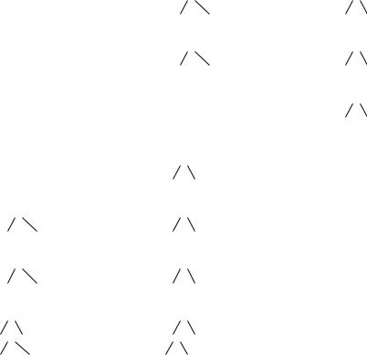
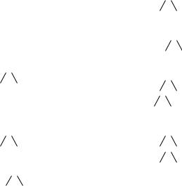
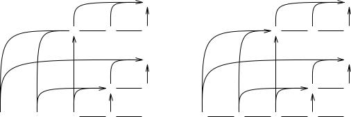
The configurations of the depth-first parser can be combined into a single graph; see Figure 7.7(a) where numbers indicate the order in which the various shifts and reduces are performed. Shifts are represented by lines to the right and reduces by upward arrows. Since a reduce often combines a number of symbols, the additional symbols are brought in by arrows that start upwards from the symbols and then turn right to reach the resulting non-terminal. These arrows constitute at the same time the partial parse tree for that non-terminal. Start symbols in the right-most column with partial parse trees that span the whole input head complete parse trees.

8 S

	a		a		a
		1		2

(a)

		11	S
9	a	10	b				3	S
		7	S
5	S	6	b
3	a	4	b	a	1	a	2	a

(b)

		11	S
5	a	9	b
		10	S
6	S	8	b
4	a	7	b

Figure 7.7 The configurations of the parsers combined

If we complete the stacks in the solution sets in our breadth-first parser by appending the rest of the input to them, we can also combine them into a graph, and, what is more, into the same graph; only the action order as indicated by the numbers is different, as shown in Figure 7.7(b). This is not surprising, since both represent the total set of possible shifts and reduces; depth-first and breadth-first are just two different ways to visit all nodes of this graph. Figure 7.7(b) was drawn in the same form as Figure 7.7(a); if we had drawn the parts of the picture in the order in which they are executed by the breadth-first search, many more lines would have crossed. The picture would have been equivalent to (b) but much more complicated to look at.

7.1.4 A slightly more realistic example

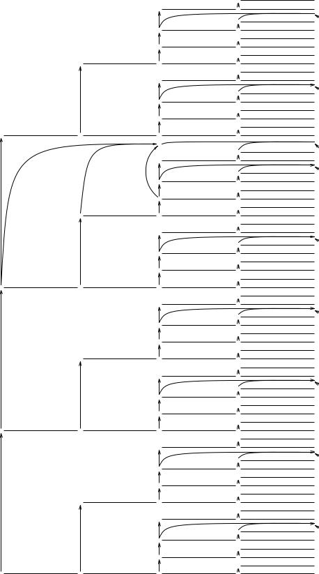
The above algorithms are relatively easy to understand and implement† and although they require exponential time in general, they behave reasonably well on a number of grammars. Sometimes, however, they will burst out in a frenzy of senseless activity, even with an innocuous-looking grammar (especially with an innocuous-looking grammar!). The grammar of Figure 7.8 produces algebraic expressions in one variable, a, and two operators, + and -. Q is used for the operators, since O (oh) looks too much like 0 (zero). This grammar is unambiguous and for a-a+a it has the correct production tree

† See, for instance, Hext and Roberts [CF 1970] for Domolki’s method to find all possible reductions simultaneously.

Sec. 7.1]

Parsing by searching

149

+

-a

a a

which restricts the minus to the following a rather than to a+a. Figure 7.9 shows the graph searched while parsing a-a+a. It contains 108 shift lines and 265 reduce arrows and would fit on the page only thanks to the exceedingly fine print the phototypesetter is capable of. This is exponential explosion.

SS -> E

E -> E Q F

E -> F

F -> a

Q -> +

Q -> -

Figure 7.8 A grammar for expressions in one variable

7.2 TOP-DOWN RESTRICTED BREADTH-FIRST BOTTOM-UP PARSING

In spite of their occasionally vicious behaviour, breadth-first bottom-up parsers are attractive since they work on-line, can handle left-recursion without any problem and can generally be doctored to handle ε-rules. So the question remains how to curb their needless activity. Many methods have been invented to restrict the search breadth to at most 1, at the expense of the generality of the grammars these methods can handle; see Chapter 9. A method that will restrict the fan-out to reasonable proportions while still retaining full generality was developed by Earley [CF 1970].

7.2.1 The Earley parser without look-ahead

When we take a closer look at Figure 7.9, we see after some thought that many reductions are totally pointless. It is not meaningful to reduce the third a to E or S since these can only occur at the end if they represent the entire input; likewise the reduction of a-a to S is absurd, since S can only occur at the end. Earley noticed that what was wrong with these spurious reductions was that they were incompatible with a top-down parsing, that is: they could never derive from the start symbol. He then gave a method to restrict our reductions only to those that derive from the start symbol. We shall see

that the resulting parser takes at most n 3 units of time for input of length n rather than

C n .

Earley’s parser can also be described as a breadth-first top-down parser with bottom-up recognition, which is how it is explained by the author [CF 1970]. Since it can, however, handle left-recursion directly but needs special measures to handle ε- rules, we prefer to treat it as a bottom-up method.

We shall again use the grammar from Figure 7.8 and parse the input a-a+a. Just as in the non-restricted algorithm, we have at all times a set of partial solutions which is modified by each symbol we read. We shall write the sets between the input symbols

150	General bottom-up parsing

			Q
		S	+
			Q
		E	+
			Q
		F	+
			Q
	Q	a	+
			Q
		S	+
			Q
		E	+
			Q
		F	+
			Q
S	-	a	+
		E
			Q
		S	+
			Q
		E	+
			Q
		F	+
			Q
	Q	a	+
			Q
		S	+
			Q
		E	+
			Q
		F	+
			Q
E	-	a	+
			Q
		S	+
			Q
		E	+
			Q
		F	+
			Q
	Q	a	+
			Q
		S	+
			Q
		E	+
			Q
		F	+
			Q
F	-	a	+
			Q
		S	+
			Q
		E	+
			Q
		F	+
			Q
	Q	a	+
			Q
		S	+
			Q
		E	+
			Q
		F	+
			Q
a	-	a	+

[Ch. 7

aFES aFES

EFES

aFES aFES aFES aFES

aFES aFES

aFES a

EFES aFES aFES aFES

aFES aFES

a

E

aFES aFES

EFES aFES

aFES aFES

aFES

aFES aFES

aFES a

EFES aFES

aFES

aFES aFES

aFES aFES

aFES a

EFES aFES

aFES

aFES aFES

aFES aFES

aFES a

EFES aFES

aFES

aFES

aFES aFES

aFES

aFES a

EFES aFES

aFES aFES

aFES aFES aFES

aFES a

EFES aFES aFES

aFES aFES aFES

a

Figure 7.9 The graph searched while parsing a-a+a