Brown M.Topology management in rooftop wireless networks.2004

The Highly Dynamic Destination-Sequenced Distance Vector (DSDV)[26] protocol is a link state routing protocol. Unlike AODV and DSR the DSDV protocol maintains a full routing table on each node in the wireless network at all times. This table is populated via hello messages sent by each node at regular intervals. When sending a hello message each node includes information regarding nodes it knows how to reach and how many hops it would take to reach them. In this way the routing table is propagated across the entire network.

A Linux implementation of the DSR and DSDV routing protocols is available through the Click Modular Router[16]. The Click implementations of DSR and DSDV have been modified to support additional routing metrics such as ETX described in Section 2.4.2. Both DSR and DSDV are able to be run at the link layer or the network layer. When running at the link layer only a single interface is supported.

OSPF

The Open Shortest Path First (OSPF)[24] routing protocol is designed for use on any IP network and has no specific features for use on wireless networks. Similar to AODV and DSDV, OSPF utilises hello messages to discover and maintain links with the direct neighbours of a node. In addition to the regular hello messages each node generates link state advertisements that are propagated to all nodes in the network whenever a link changes state. Each link in an OSPF network has an associated metric which is traditionally based on the bandwidth of the link. For each possible route to a destination a node calculates the sum of the link metrics in that path. The path with the lowest sum is chosen as the best route.

OSPF is a widely used routing protocol and has a mature Linux implementation as a part of the Quagga[30] routing suite. The Quagga routing suite is a set of programs that provide a variety of routing protocols to Linux and other Unix based operating systems. Quagga uses an interface layer between the kernel and the logic of the routing protocol to make it easy to modify and create new routing protocol implementations. The CRCnet project currently uses the Quagga OSPF implementation for the network described in Section 1.3.

2.5Design Requirements

After reviewing existing 802.11b networks and available routing protocols the following design requirements were reached for the mesh network to be constructed by this project. These requirements also draw on the experience gained from building and managing CRCnet. Figure 2.3 shows the topology of an example mesh network similar to what this project would like to create.

The mesh network must ensure that every mesh node that is within communication range can communicate with all other nodes in the mesh. This communication must be achieved with a high level of performance and redundancy as described in section 1.4. Given the limitations of the 802.11 MAC protocol the mesh network

14

Figure 2.3: Example mesh network showing all possible links

should favour point to point links in ad-hoc mode to maximise performance. Some situations may require the use of point to multi point, or even multi point to multi point links to ensure that all nodes are connected to the network in a redundant measure. While this is acceptable to achieve the desired level of connectivity, point to point links should be used whenever possible.

The mesh network should utilise multiple wireless interfaces on each node, coupled with directional antenna to increase the overall capacity available to the network. The use of directional antenna also reduces the level of interference between links which allows denser networks to be constructed. A node with four wireless interfaces should be able to effectively communicate in all directions using a directional antenna on each interface. The use of multiple interfaces also increases the ability of each node to form point to point links with other nodes.

The implementation of the mesh network must be modular to allow for future development of the protocol without having to completely redesign it. For example while all development for this project will take place with 802.11b wireless cards, moving to 802.11g wireless cards should require only minimal changes to the implementation. The mesh network should also seek to reuse existing utilities and open source software such as the Linux kernel and the Quagga routing suite to lower development time as much as possible. Given the lack of access to the control software of the wireless cards the implementation must not require modifications to the 802.11b MAC layer.

15

Chapter 3

Mesh Protocol

This chapter describes the protocol that has been implemented by this project to create a mesh network with the characteristics described in Sections 1.4 and 2.5.

3.1Protocol Aim

The aim of the mesh protocol is to take a set of independent nodes and form them into a mesh network. Each node in the network operates autonomously and the protocol must not rely on any form of centralised control. The protocol specifies the tasks each node must perform and how to perform them.

Each node in the mesh network must have a unique identifier, called the Node ID, and at least one wireless interface with which it can communicate with other mesh nodes. Multiple interfaces on a mesh node must be assigned an index to allow them to be uniquely identified in the mesh network.

3.2Protocol Tasks

Creating a mesh network from a set of independent nodes requires each node to undertake four basic tasks, Neighbour Discovery, Neighbour Selection, Link Establishment and Routing. These tasks must be completed in order as each task relies on the results of the previous one. Tasks 1 and 3 are performed individually on each interface of a node, while tasks 2 and 4 operate on information gained from all interfaces of a node.

Each mesh node must discover if there are any other mesh nodes within its communication range before it can perform any other step. The process of finding other nodes within communication range is called neighbour discovery.

After performing neighbour discovery it is likely that a mesh node will have multiple choices in links to another mesh node. Neighbour selection involves choosing a subset of all possible links to be configured and become part of the mesh.

16

Once the node has selected the links to establish, the parameters of each link must be agreed upon with each neighbour node. Ensuring that each node is synchronised is crucial to the success of link establishment.

As the links in the mesh network are established, a routing protocol must calculate the best paths through the network and setup the routing table on each node.

The four tasks can be used to loosely describe the state of each interface on a node at any point in time. There is no requirement for all interfaces on a node to be in the same state at once, and an interface must be able to respond correctly to any packets that it receives regardless of it’s current state.

3.3Hello Protocol

Each of the tasks described in the previous section requires some level of information to be transfered or collected from neighbour nodes in the mesh network. Building on the techniques used in the AODV and OSPF routing protocols described in Section 2.4, a hello protocol is used for neighbour discovery, synchronisation and link maintenance in the mesh protocol.

3.3.1 Hello Packets

The operation of the hello protocol centres around the transmission of a hello packet every five seconds from each interface of a mesh node. Hello packets are always padded to 1500 bytes long to avoid the problems encountered in the AODV protocol described in Section 2.4.3. Additionally hello packets are directed to a specific neighbour node rather than being sent to the broadcast address to ensure that they are treated identically to normal data packets. In situations where an interface has no neighbour nodes (such as during neighbour discovery) the hello packet can be sent to the broadcast address.

0			1	2		3
0 1 2 3 4 5 6 7 8 9 0 1 2 3 4 5 6 7 8 9 0 1 2 3 4 5 6 7 8 9 0 1
+---------------		+	---------------	+---------------	+	---------------	+
|				Node ID			|
+---------------		+---------------		+---------------	+---------------		+
|	IfaceID	|	Seq No	| LSR Count	|	IF State	|
+---------------		+---------------		+---------------	+---------------		+
|							|
.			Link State Records				.
.							.
.							.
+---------------		+---------------		+---------------	+---------------		+

Figure 3.1: Hello Packet Format

Each hello packet contains the following pieces of information as shown in figure 3.1.

17

Node ID (4 bytes) – The unique identifier of the node that generated the hello packet .

IfaceID (1 byte) – The index of the interface on the node that generated the packet. Combined with the previous Node ID field this uniquely identifies where the hello packet came from.

Seq No (1 byte) – A sequence number that is incremented with every hello packet sent from the interface. This allows neighbour nodes to determine if a hello packet has been lost.

LSR Count (1 byte) – A count of the number of Link State Records (LSRs) contained in the second half of the hello packet.

IF State (1 byte) – The state of the interface that generated the hello packet at the time it was sent.

Link State Records (variable length) – A series of records of the format shown in Figure 3.2 describing each link in the sending nodes link database. The number of records in this section is specified by the LSR Count field.

The primary function of a hello packet is to allow the receiver node to determine that the sender node is still online. If a three consecutive hello packets are not received from a neighbour node it is assumed to be down and the interface will return to neighbour discovery mode.

The secondary function of the hello packets is to synchronise the link database on each node via the link state records contained in the second half of the hello packet.

0	1	2	3
0 1 2 3 4 5 6 7 8 9 0 1 2 3 4 5 6 7 8 9 0 1 2 3 4 5 6 7 8 9 0 1
+---------------	+---------------	+---------------	+---------------	+
|	Node 1 Id			|
+---------------	+---------------	+---------------	+---------------	+
|	Node 2 Id			|
+---------------	+---------------	+---------------	+---------------	+
| N1 Iface ID	| N2 Iface ID	| LSR Seq. No.	| No. Channels	|
+---------------	+---------------	+---------------	+---------------	+
|	LSR Originator ID			|
+---------------	+---------------	+---------------	+---------------	+
.				.
.	Channel Information			.
.				.
+---------------	+---------------	+---------------	+---------------	+

Figure 3.2: Link State Record Format

Each link state record contains the following pieces of information as shown in figure 3.2.

Node 1 ID (4 bytes) – The unique identifier for the first node that is part of the link.

18

Node 2 ID (4 bytes) – The unique identifier for the second node that is part of the link.

N1 Iface ID (1 byte) – The index of the interface on the first node that is part of the link.

N2 Iface ID (1 byte) – The index of the interface on the second node that is part of the link.

LSR Seq. No (1 byte) – A sequence number that is incremented every time a new LSR for this link is origi-

nated. This enables LSRs to be expired when the node originating them has left the mesh network.

No. Channels (1 byte) – The number of channel records contained in the second half of the packet.

LSR Originator ID (4 bytes) – The unique identifier for the node that originated this LSR.

Channel Information (variable length) – A series of records of the format shown in Figure 3.3 describing

the channels that have been tested or are in use for this link.

Each link state record contains a number of channel information records that describe the quality of that

channel, and its current state. Each field in a channel information record is described below and illustrated in

Figure 3.3.
0	1
0 1 2 3 4 5 6 7 8 9 0 1 2 3 4 5

+---------------+---------------+ | Chann | State | Quality | +---------------+---------------+

Figure 3.3: Channel Information Record Format

Chann (4 bits) – 802.11b channel number that this record relates to.

State (4 bits) – The current state of the channel. Valid values are:

2 (Active) – The channel is currently in use.

1 (Chosen) – The channel has been chosen for use but is not yet active.

0 (Available) – The channel is available for use.

Quality (1 byte) – The signal quality of the link on the specified channel as reported by the radio card. This value is updated with each hello packet that is received on the link.

3.4Link Database

Each node in the network maintains a link database which describes all possible links between nodes in the network. The link database is populated with the information each interface reports about its directly

19

connected neighbours and from the link state records contained in received hello packets. When a new link entry is added to the link database it is given a timestamp. Each time a new link state record is received the originating node ID and the sequence number of the new record are checked against the database. If the originating node ID matches and the sequence number has increased the timestamp is updated, otherwise the new link record is discarded. Link entries related to directly connected neighbours are also regularly updated from the nodes interfaces. If the timestamp of an entry is not updated for seven consecutive hello intervals the entry is removed from the database.

3.5Neighbour Discovery

The following procedure is carried out by a mesh node on each of its interfaces that is not currently part of an established link. If no neighbours are discovered when the procedure is initially carried out it is repeated every thirty seconds until a neighbour is discovered. In-between these repetitions of the procedure the node will transmit hello packets to the broadcast address so that any new nodes coming on line can hear the hello packet and respond.

3.5.1 802.11 Network Discovery

The 802.11 specification defines a procedure called a scan, in which the radio card very quickly monitors every channel and reports back a list of any active 802.11 networks that were found. This procedure is usually used by devices such as laptops to find access points, however there is no technical restriction on how it can be used. Performing a scan takes two to three seconds and returns a list of all 802.11 networks in the area. Other information such as the estimated signal strength of each network is also present in the response. This information provides an excellent first step in determining if there are any mesh nodes nearby, however it will also pick up 802.11 networks that are completely unrelated to the mesh. A filtering step to remove these unwanted results is needed.

3.5.2 Scan Result Filtering

To remove 802.11 networks that are not part of the mesh a two step filtering process is performed on the results of the 802.11 scan. Every link established by the mesh network has a string prepended to the start of its name. The first step in filtering the results of the 802.11 scan involves removing any network that does not begin with the correct string. After this step has been completed there is a fairly high chance that any remaining 802.11 networks belong to a mesh node, however a further check is needed to ensure that a laptop (or some other device) has not automatically associated itself with a mesh network node and is continuing to use the network name even after the mesh node has gone away.

20

The second filter step involves sending a probe packet onto each detected network. Any mesh node receiving a probe packet must immediately send a hello packet in response. If the node performing neighbour discovery does not receive a response to the first probe packet it will continue to send probe packets at five second intervals until a total of five probe packets have been sent. If no response is received in this time the node will assume that no valid mesh nodes exist on that network and discard it from the results. If a response to a probe is received the node updates the link database with the contents of the received hello packet and waits for the results of the neighbour selection algorithm described in the next section before proceeding further.

3.6Neighbour Selection

After completing the neighbour discovery phase the mesh node must determine the desired topology of the mesh network in order to know how to configure each of its interfaces. The darker nodes and links in Figure 3.4 show the information that node A possesses about its neighbour nodes and the possible links that could be formed after completing the neighbour discovery step. In many cases there are several links that node A could form in order to communicate with a specific neighbour node.

Figure 3.4: Node A’s view of network after neighbour discovery

The task of the neighbour selection algorithm is to determine which links should be established and consequently the topology of the mesh network. This step is crucial to the performance of the mesh network as all further use of the network is constrained by the quality of the links that are chosen to be established in this step.

To maintain a reliable network provision should be made so that the failure of a single node can be accepted without taking any other nodes off line. This level of reliability can be achieved by making sure that there are multiple redundant paths between any two nodes. In the event of a node in the first path failing the traffic is simply routed over the second path.

21

Creating redundant paths through the mesh to increase reliability requires that mesh nodes be densely located so that many possible links are available for the neighbour selection algorithm to choose from. Unfortunately the closer the mesh nodes are to each other the higher the chance that their performance will be degraded by interference between them. This problem is aggravated when extra links are added to provide redundancy.

3.6.1 Spanning Tree Based Neighbour Selection

This project has implemented a neighbour selection algorithm that is based on the principle of a minimal spanning tree. The list of edges that can be used to build the spanning tree is built by extracting every link in the link database and computing a cost for each one. The cost of a link is calculated from the best signal quality that is available for that link and a factor based on the current state of the link. The factor favours links that are currently active in the mesh to provide stability. The list is sorted such that currently active links with the highest quality are first.

The spanning tree is built by iterating over the list of links in order and adding them to the tree until it contains N-1 links, where N is the number of mesh nodes in the link database. This ensures that all nodes in the network are connected without providing any redundancy. When building the spanning tree only point to point links are used so that each interface on a node is part of a single link. If the end of the list of links is reached before N-1 point to point links have been added to the tree the process is repeated from the start of the list with the point to point requirement modified so that a point to multi point link may be created if it connects a node that is currently isolated.

Figure 3.5 shows an example spanning tree network topology that could be created from the network shown in Figure 3.4 once all nodes have completed neighbour discovery. The spanning tree approach ensures that all mesh nodes are connected by high quality links fulfilling the two important design requirements of the mesh network.

3.6.2 Redundant Links

After the spanning tree has been constructed the algorithm performs three further iterations over the remaining links in the list. Each iteration reduces the quality that is required of a link in order for it to be added to the tree. The criteria applied to each link in the three iterations are shown in the following list.

1.Point to point links with high signal quality

2.Point to multi point links with high signal quality

3.Multi point to multi point links with high signal quality

22

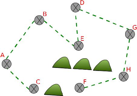
Figure 3.5: Example spanning tree network topology

This process transforms the spanning tree into a network graph that can be presented to the rest of the mesh protocol and ensures that the redundant links added to the mesh are of the highest possible quality. The algorithm stops at the end of the three iterations or when one of the following two conditions is met.

1.Every interface that has neighbours is part of a link, or

2.Each node has a link to at least two different neighbours

After completing this step the spanning tree network shown in Figure 3.5 will have been transformed into a complete mesh network as shown in Figure 3.6.

3.6.3 Channel Allocation

Each link that is selected to be part of the mesh network is assigned a channel by the neighbour selection algorithm. The algorithm implemented by this project uses a random scheme to allocate channels. The algorithm tries to ensure that each node does not use the same channel on more than one interface to avoid interference. The algorithm utilises all fourteen 802.11b channels but has no knowledge of which channels overlap. An attempt is made to use the channel that the link was initially discovered on but this may not be possible if two interfaces on a node discovered links on the same channel.

23