Carr D.M.PID control and controller tuning techniques

The following is a reprint of the copyrighted article about Eurotherm’s PID control. All rights strictly reserved. No part of this document may be stored in a retrieval system, or any form or by any means without prior written permission from Eurotherm Controls Inc. Every effort has been taken to ensure the accuracy of this specification.

AN-CNTL-13

PID CONTROL AND CONTROLLER TUNING TECHNIQUES

Version 1

D. Mitchell Carr

April 23, 1986

Proper tuning of a controller is not only essential to its correct operation but will also greatly improve product quality, reduce scrap, shorten down-time and save money. Procedures for tuning conventional PID controllers are well established and simple to perform. Any time a controller is replaced, the new instrument must be retuned, which can be difficult under certain running conditions. Some controllers have digital settings for the three control parameters: Proportional Band, Integral time constant and Derivative time constant. This feature makes it simple to reproduce the correct parameter settings when replacing an instrument but does not help if heaters are changed or the mechanics of the system are altered appreciably. In this instance the associated controller must be "re-tuned" to insure optimal performance.

PID Control

Most conventional temperature controllers, whether analog or microprocessor-based, are three-term, PID, controllers. That is to say that the control algorithm is based on a proportional gain, an integration action and a derivative action. Occasionally a relative cool gain adjustment is available and, on more refined instruments, a parameter for overshoot inhibition may be present. What are these things and what do they do?

SETPOINT

TEMPERATURE

TIME

FIGURE 1: PROPORTIONAL-ONLY CONTROL

Gain, or as it is more commonly called, Proportional Band, simply amplifies the error between setpoint and measured value to establish a power level. The term Proportional Band is one that expresses the gain of the controller as a percentage of the span of the instrument. A 25% PB equates to a gain of 4; a 10% PB is a gain of 10. Given the case of a controller with a span of 1000 degrees, a PB of 10% defines

1

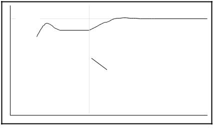
a control range of 100 degrees around setpoint. If the measured value is 25 degrees below setpoint, the output level will be 25% heat. The Proportional Band determines the magnitude of the response to an error. If the Proportional Band is too small, meaning high gain, the system will oscillate through being over-responsive. A wide Proportional Band, low gain, could lead to control "wander" due to a lack of responsiveness. The ideal situation will be achieved when the Proportional Band is as narrow as possible without causing oscillation. Figure l shows the effect of narrowing the Proportional Band to the point of oscillation. This control zone comes up to temperature with a 25% Proportional Band but there is an appreciable error between setpoint and actual temperature. As the Proportional Band is reduced, the temperature comes closer to setpoint until finally, at a setting of 1.5% the system becomes unstable.

Integral action, or Automatic Reset, is probably the most important factor governing control at setpoint. The integral term slowly shifts the output level as a result of an error between setpoint and measured value. If the measured value is below setpoint the integral action will gradually increase the output power level in an attempt to correct this error. Figure 2 demonstrates the result of introducing Integral action. Again the temperature rises and levels out at a point just below setpoint. A 6% Proportional Band is used. Once the temperature settles, Integral action is introduced. Notice that the temperature rises further until it is at setpoint. The adjustment of this term is usually expressed in one of two ways; as a time constant in either minutes or seconds, or, the inverse of a time constant expressed as repeats/minute. If it is expressed as a time constant, the longer the Integral time constant, the more slowly the power level will be shifted (the fewer repeats/min., the slower the response). If the Integral term is set to a fast value the power level could be shifted too quickly thus causing oscillation since the controller is trying to work faster than the load can change. Conversely, an Integral time constant which is too long will result in very sluggish control. In Figure 3a, a Proportional Band of 6% and an Integral time constant of 200 seconds provides stable control at setpoint. A positive 20 degree perturbation results in some overshoot before settling. Figure 3b shows the result of a similar perturbation but with a 400 second Integral time constant. Lengthening the Integral time constant results in the markedly slower response shown.

	SETPOINT
TEMPERATURE	PROPORTIONAL-INTEGRAL
	CONTROL
	PROPORTIONAL-
	ONLY CONTROL
	INTEGRAL
	ADDED
	TIME

FIGURE 2: ADDING INTEGRAL ACTION

Derivative action, or Rate, provides a sudden shift in output power level as a result of a quick change in measured value. If the measured value drops quickly the derivative term will provide a large change in output level in an attempt to correct the perturbation before it goes too far. Derivative action is probably the most misunderstood of the three. It is also the most beneficial in recovering from small perturbations. The oscillatory response to a perturbation shown in Figure 4a is virtually eliminated by Derivative action as shown in Figure 4b where a 40 second Derivative term is added to the 6% Proportional Band and 200 second Integral time constant. As with the other two tuning parameters, there is a way of improperly setting this term. Derivative oscillation is typically a cyclic wander away from setpoint. The Derivative time constant is usually set to a value equal to one sixth of the Integral time constant.

2

o	FIGURE 3a	FIGURE 3b
20
TEMPERATURE	SETPOINT
o	8 minutes	8 minutes
20
-	INTEGRAL TIME CONSTANT	INTEGRAL TIME CONSTANT
	200 SECONDS	400 SECONDS

FIGURE 3: WIDENING INTEGRAL TIME CONSTANT

o	FIGURE 4a	FIGURE 4b
20
TEMPERATURE	SETPOINT
o	8 minutes	8 minutes
20
-	PROPORTIONAL-INTEGRAL	RESPONSE WITH 40 seconds
	CONTROL RESPONSE	DERIVATIVE ACTION

FIGURE 4: ADDING DERIVATIVE ACTION

Derivative action, when used, is often mistakenly associated with overshoot inhibition rather than transient response. In fact Derivative should not be used to curb overshoot on start-up. To effectively use Derivative to prevent overshoot on start-up the steady-state performance must be greatly degraded. Some new micro-processor-based controllers contain a separate parameter which can be adjusted to prevent overshoot. This parameter, often labeled Approach control, is independent of the other three tuning values and in no way affects their performance. Figures 5a and 5b are chart recordings of start-up curves for the same load; the PID tuning values are identical in each case, but, the Approach control parameter is set to a much more effective value in Figure 5b. By using a variable overshoot-inhibition parameter, the system can be set up for optimum steady state response and the overshoot can be limited as desired.

3

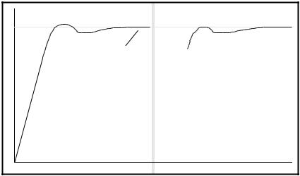
FIGURE 5a	FIGURE 5b
SETPOINT
TEMPERATURE
WITHOUT OVERSHOOT	WITH OVERSHOOT
SUPPRESSION	SUPPRESSION

FIGURE 5: OVERSHOOT SUPPRESSION

No matter how thorough the explanation of PID control and the function of each of the three parameters, there is always some confusion over how it all ties together. A few common questions seem to pop up repeatedly and they should be highlighted here:

1.Why does my controller continue to call for heat even though the actual temperature is above setpoint?

A PID controller behaves in a very smooth and gradual way, making subtle changes to take care of small deviations, and large, short duration, changes to correct for rapid perturbations; it is NOT an ON-OFF controller. A person driving a car can be used as an example of a PID controller; if the driver realizes that he is slightly above the speed limit, he will gradually decrease the pressure he is exerting on the accelerator pedal. This is an example of Integral action slowly shifting the output to correct for a small] problem. If, however, the driver spots a police radar trap at the same time that he notices he is speeding, he will slam on the brakes to keep from getting a ticket. This is an example of Derivative action injecting a large change in output to prevent a sudden change from getting out of hand.

In considering the example of the driver in a car exceeding the speed limit; the driver will decrease the speed of the car gradually by reducing the pressure on the accelerator pedal slightly. Similarly, if the PID controller recognizes an over-temperature condition, it will decrease the heat demand slightly to bring the temperature down. In reflecting on the initial question, “Why does my controller continue to call for heat even though the actual temperature is above setpoint?”; if the controller shut off the heat completely the temperature would drop to ambient just as the driver of a car stepping on the brake pedal causes the car to stop.

2.On start-up, why does the heat output level begin decreasing before the measured value reaches setpoint?

If 100% heat is applied to the load continuously until the measured value has reached setpoint, the temperature will overshoot considerably. Power must be cut back before the temperature reaches setpoint, sometimes well before, to prevent overshoot. Again, using the analogy of the driver in a car; if the car is standing still and you would like to drive at 55 MPH, you do not press the accelerator to the floor until you reach 55 MPH, then slack off. This would surely result in a maximum speed in excess of 55 MPH. Many heat loads love to overshoot on start-up and to curb this, the output level must begin decreasing well in advance.

Each implementation of the PID algorithm behaves in a slightly different manner due to the subtle variations in the controller’s algorithm, circuitry or programming. Some controllers provide excellent

4

overshoot inhibition as an inherent quality or perhaps superior response to setpoint changes. These are the factors which make one controller better than the next In addition, the introduction of microprocessors has helped to enhance the flexibility of controllers. Whereas before, overshoot inhibition, for instance, might have been built into an analog controller in an unalterable way, it can now be an adjustable parameter. There is no standardization, however, in setting overshoot inhibition parameters as each instrument manufacturer employs a different method.

Classical Tuning Techniques

There are several established techniques for tuning control loops. The two most common are the Process Reaction Curve technique and the Closed-Loop Cycling method. These two methods were first formally described in an article by J.G. Ziegler and N.B. Nicholls in 1942 (1). They were initially proposed as being equal in their ability to be used for tuning but, as will be seen, one technique is superior to the other.

It should also be understood that “optimal tuning”, as defined by J.G. Ziegler and N.B. Nicholls is achieved when the system responds to a perturbation with a 4:1 decay ratio. That is to say that, for example, given an initial perturbation of +40 degrees, the controller’s subsequent response would yield an undershoot of -40 degrees followed by an overshoot of +2.5 degrees. This definition of “optimal tuning” may not suit every application, so the trade-offs must be understood.

P

OUTPUT LEVEL

TEMPERATURE

Line drawn through

point of inflection

R

L

TIME

FIGURE 6: PROCESS REACTION CURVE - SIMPLE

5

Process Reaction Curve

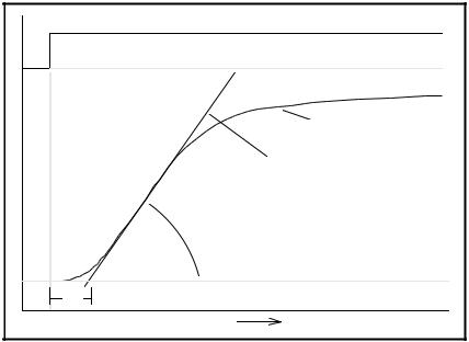
The Process Reaction Curve is obtained by removing the controller from the circuit and injecting a step input of power. The power level injected can be any convenient, safe amount, but should be introduced when the system is stable at room temperature. A chart recorder should be used to obtain a graph of the measured value similar to that shown in Figure 6.

The time, L, is often referred to as the Lag Time and is considered to be the time necessary to overcome the thermal inertia of the load being heated. A straight line drawn tangent to the Process Reaction Curve at the point of inflection will have a slope, R. From these two terms, the PID values may be calculated by the equations below.

Pb = (RL P) × (100% (span))	Proportional Band is expressed as percent of instrument span
	whereas TI (integral) and TD (derivative) are time constants
	expressed in minutes.
TI = 2L	P is the percent power level used as the step input divided by 100%
	(expressed as a fraction).

Further work attributed to G. H. Cohen and G. A. Coon (2), yielded a more thorough evaluation of the Process Reaction Curve (Figure 7).

T = Final attained temperature expressed as a percent of span of the instrument as a result of the step input P.

P = Step input of power used for the evaluation expressed as a percent of maximum allowable power.

K = T P

Again it should be noted that the goal here is to achieve a 4:1 decay ratio, which may not be suitable for all applications. To reduce overshoot and lengthen settling time, increase Proportional Band and the Integral time constant.

CONTROLLER

PROPORTIONAL

INTEGRAL TIME

DERIVATIVE TIME

BAND Pb

CONSTANT TI

CONSTANT TD

PROPORTIONAL

K t1

NOT

NOT

ONLY

( P )

t2 ( 1+ t1/3 t2 )

APPLICABLE

APPLICABLE

PROPORTIONAL

K t1

t1 (30+ 3 t1/ t2 )

NOT

and INTEGRAL

APPLICABLE

t2 (0.9+ t1/2 t2)

9 + 20 t1/ t2

( P I )

PROPORTIONAL

K t1

NOT

t1 (6 - 2 t1/ t2 )

and DERIVATIVE

APPLICABLE

(1.25 t2 + t1/ 6 )

22 + 3 t1/ t2

( P D )

PROPORTIONAL

K t1

t1 (32 + 6 t1/ t2 )

4 t1

INTEGRAL and

DERIVATIVE

t2 (1.3 + t1/ 6 t2 )

13 + 8 t1/ t2

11 + 2 t1/ t2

( P I

D )

TABLE 1: PROCESS REACTION CURVE TUNING CONSTANTS

6

P	OUTPUT LEVEL
T
	TEMPERATURE
	Line drawn through
	point of inflection
T1	T2
	TIME

FIGURE 7: PROCESS REACTION CURVE - EXPANDED

T

SETPOINT

FIGURE 8: CLOSED-LOOP CYCLING

Closed Loop Cycling

By placing a Proportional-only controller (no Integral or Derivative terms in oscillation by setting the Proportional Band to a very small value, the control loop will cycle with a characteristic frequency (Figure 8). This characteristic frequency will be a very accurate representation of the system’s responsiveness and therefore can be used to derive the controller time constants. To outline procedure:

1.Eliminate Integral and Derivative action from the controller .

2.Reduce the Proportional Band until the control loop oscilllates. Measure the period of oscillation, T.

3.Widen the Proportional Band until the process is just slightly unstable. This value of Proportional Band, is referred to as the point of ultimate sensitivity.

4.Refer to the Table 2 for values of Pb, TI and TD.

7

	CONTROLLER		PROPORTIONAL	INTEGRAL TIME	DERIVATIVE TIME
			BAND Pb	CONSTANT TI	CONSTANT TD
	PROPORTIONAL		2 P	NOT	NOT
	ONLY	( P )		APPLICABLE	APPLICABLE
	PROPORTIONAL		2.2 P		NOT
	and INTEGRAL			0.8 T	APPLICABLE
	( P	I )
	PROPORTIONAL
	INTEGRAL and		1.67 P	0.5 T	0.12 T
	DERIVATIVE
	( P I	D )

TABLE 2: CLOSED-LOOP CYCLING TUNING CONSTANTS

Again, the settings given in the chart establish control with a 4:1 decay ratio which may give too much overshoot for some processes. Table 3 gives guidelines for altering these values, when using Proportional, Integral and Derivative terms.

	CONTROLLER	PROPORTIONAL	INTEGRAL TIME	DERIVATIVE TIME
		BAND Pb	CONSTANT TI	CONSTANT TD
	UNDER-DAMPED	P	0.5 T	0.125 T
	CRITICALLY	1.5 P	T	0.167 T
	DAMPED
	OVER-DAMPED	2 P	1.5 T	0.167 T

TABLE 3: VARYING RESPONSE - TUNING CONSTANTS

START-UP RESPONSE	PERTURBATION RESPONSE
UNDER-DAMPED RESPONSE
CRITICALLY DAMPED
RESPONSE
OVER-DAMPED RESPONSE

FIGURE 9: TYPICAL RESPONSE CURVES

Forced Cooling

8

Certain loads require some form of forced cooling action, used either to overcome the heat generated by an exothermic process or to bring the temperature of the load below ambient temperature. In these cases, cooling action is achieved either by cycling a fan or blower motor or by pulsing a cooling liquid such as oil or water through the system. Two things must be considered to insure proper cooling action; that the cooling source is driven correctly and that the control loop tuning is correct for the system when using cooling.

Linear Versus Non-Linear Cooling

Systems which employ forced air for cooling are very linear in response. Additional cooling is supplied by cycling the fan or blower on for a greater percentage of the time. There are a number of systems which use pulsed water for cooling a load which is at a temperature above the boiling point. A system such as this behaves with a very non-linear characteristic. As a small amount of cooling, short pulses of water, is applied, the water will flash off to steam thus extracting a great deal of heat from the load due to the latent heat of vaporization. The slightest increase in cooling water flow will result in a drastic change in cooling action. For this reason, the gain of the system should be very low for this condition. As the amount of cooling demanded by the system increases, the flow of water will increase to the point where the water is not flashing off to steam but is flowing. In this instance, changes in cooling action do not have as great an effect as before and thus the gain of the controller must be increased to compensate for the change in the cooling characteristic. Controllers are available with non-linear cooling output characteristics specifically designed to compensate for this problem. (See Figure 10.)

100%

OUTPUT CYCLING

0%

0%

OUTPUT DEMAND

100%

FIGURE 10: NON-LINEAR WATER COOLING CHARACTERISTIC

Relative Cool Gain

As the cooling action is separate and distinct from the heating action, it will have a very different effect and magnitude in most cases. That is to say that if there is 10KW of heating available, there may be 20KW of cooling. If the controller is tuned for proper heating action (which is the case, usually) it will have an incorrect gain setting for the cooling action. Since cooling action is typically applied at the same location as the heating action, the load time constants will be the same but since the magnitude is different then the gain will be wrong. For this reason, heat/cool controllers offer a relative cool Gain adjustment. The Relative Cool Gain adjustment is a multiplier for the Proportional Band that is used

9

when the controller is delivering cooling power. In the example case, above, if there is 10KW of heating available but 20KW of cooling, the heating Proportional Band will be inappropriate for the cooling action; the controller will oscillate from too much cooling action. In this case, the Relative Cool Gain adjustment should be set to a value of 0.5 which will reduce the gain by a factor of two (widen the Proportional Band) and balance the cooling with the heating.

Tuning Cooling

If there is not enough cooling action, if the Relative Cool Gain is too small, the temperature will remain above setpoint for a pro-longed period of time and will be very sluggish in dropping back to setpoint (assuming the controller is requesting cooling output. In this instance, the Relative Cool Gain should be increased. Cooling oscillation is very easily determined as the behavior is predictable and pathological. As shown in Figure 11, the temperature will slowly rise above setpoint as the power demand from the controller decreases gradually. Eventually, the cooling action will cause a rapid drop in temperature resulting in a sharp increase in power demand back into the heating region. The classic cycling between heating and cooling with this sawtooth waveform characteristic will be reduced by lowering the Relative Cool Gain adjustment.

Heat	OUTPUT DEMAND LEVEL
0%
Cool
	TEMPERATURE
	SETPOINT

FIGURE 11: COOLING OSCILLATION

Troubleshooting PID Tuning

In any instances a control loop will be slightly unstable and oscillate a few degrees. This may be due to the fact that the loop was never properly tuned or that the tuning procedures outlined above were not quite appropriate for the load. In these cases, it may not be desirable to repeat the somewhat extensive tuning procedures outlined above. To quickly “repair” the tuning of the control loop, several things may be tried. The first thing to do is compare the period of oscillation (reference Figure 8) to the Integral time constant setting; the Integral Time Constant should be at least as long as the period of oscillation. If the Integral Time Constant is shorter that the period of oscillation, it should be increased to at least that value. If the loop continues to oscillate with the appropriate integral term, the Proportional Band should be increased to eliminate the oscillation. Make sure the zone is not in cooling oscillation (Figure 11).

Some control zones have certain physical configurations which prevent them from being tuned with Derivative action. Even though Derivative action is a stabilizing factor in most heated loads, some loads have transport lags which cannot stabilize if Derivative is used. This would occur, for example, in a system where heat is transported to the load by flowing air. If adjusting the integral action and

10