Chen G.R.Fuzzy PID controllers for industrial applications

Fuzzy PID Controllers for Industrial Applications

G. Ron Chen

Lecture for EE 6452

City University of Hong Kong

Summary

∙Proportional-Integral-Derivative (PID) controllers are the most widely used controllers in industries today

∙Statistics: > 90% controllers in industries are PID or PIDtype of controllers (the rest are programmable logical controllers (PLC))

∙Merits of PID controllers: simple, cheap, reliable, and effective

∙For lower-order linear time-invariant systems and processes, PID controllers have good set-point tracking performance with guaranteed stability

∙Fuzzy logic provides a certain level of artificial intelligence to the conventional PID controllers

∙Fuzzy PID controllers have self-tuning ability and on-line adaptation to nonlinear, time -varying, and uncertain systems

∙Fuzzy PID controllers provide a promising option for industrial applications with many desirable features

Outline of the Presentation

∙Overview of the Fuzzy Logic Technology

∙Overview of Conventional PID Controllers

∙Introduction to Fuzzy PID Controllers

∙Some Successful Examples of Applications

∙Concluding Remarks

Overview of the Fuzzy Logic Technology

Closed-Loop Set-Point Tracking System

Consider the typical set-point tracking system:

r	+	Σ	e	Controller	u	Plant	y
(reference			(error		(control
							(output
	signal)	−	signal)		signal)
							signal)

Figure 1 A typical closed-loop set-point tracking system

Objective:

e(t) := r(t) − y(t) → 0 (t→∞)

Approach: Design a fuzzy logic controller (FLC)

	e	Fuzzification	Fuzzy Rule Base	Defuzzification	u
	controller				controller
	input				output
			Fuzzy Logic Controller (FLC)
		Figure 2 General structure of a fuzzy logic controller

temperature
b	c	y(t )
r = 45 o	d
e(t )
a

0				t
Figure 3 Temperature set-point tracking example
(i) If e > 0 then
e = r − y > 0	or		r > y
the output y is at position		a	or	d
(ii) Furthermore, if	e& < 0	then
e& = r& − y& = 0 − y&			or	y& > 0
(iii) Therefore, the output		y	is at position a

Fuzzy Logic Rule Base:
R1:	IF e > 0	AND e& < 0 THEN u(t+) = u(t)
R2:	IF e < 0	AND e& < 0	THEN u(t+) = − u(t)
R3:	IF e < 0	AND e& > 0	THEN u(t+) = u(t)
R4:	IF e > 0	AND e& > 0	THEN u(t+) = − u(t)

Fuzzy Controller Design

A. Fuzzification

Purpose: Enable the input physical signal to use the rule base

Approach: Use membership functions
1	μPS	μPL	μNL	μNS	1
0	H	.	−H		0	.
		e, e				e, e
		(a)	(b)
Figure 4 Four membership functions for signals e and e&

B. Programmable Rule Base

R1:	IF e = PL AND e&
R2:	IF e = PS AND e&
R3:	IF e = NL AND e&
R4:	IF e = NS AND e&
R5:	IF e = NL AND e&
R6:	IF e = NS AND e&
R7:	IF e = PL AND e&
R8:	IF e = PS AND e&

<0 THEN u(t+) = μP L(e) . u(t)

<0 THEN u(t+) = (1−μPS(e)) . u(t)

<0 THEN u(t+) = −μNL(e) . u(t)

<0 THEN u(t+) = −(1−μNS(e)) . u(t)

>0 THEN u(t+) = μNL(e) . u(t)

>0 THEN u(t+) = (1−μNS(e)) . u(t)

>0 THEN u(t+) = −μPL(e) . u(t)

>0 THEN u(t+1) = −(1−μPS(e)) . u(t)

To implement the FLC on a digital computer:

u(t) = u(kT) and u(t+) = u((k+1)T)

where T is the sampling time.

R1:	IF e(kT) = PL AND e& (kT) < 0
	THEN u((k+1)T ) = μ (e(kT)) . u(kT)
				PL
R2:	IF e(kT) = PS AND e& (kT) < 0
	THEN u((k+1)T) = (1−μ (e(kT))) . u(kT)
				PS
R3:	IF e(kT) = NL AND e& (kT) < 0
	THEN u((k+1)T ) = −μ (e(kT)) . u(kT)
				NL
R4:	IF e(kT) = NS AND e& (kT) < 0
R5:	THEN u((k+1)T ) = −(1−μNS(e(kT))) . u(kT)
	IF e(kT) = NL AND e& (kT) > 0
	THEN u((k+1)T ) = μ (e(kT)) . u(kT)
				NL
R6:	IF e(kT) = NS AND e& (kT) > 0
	THEN u((k+1)T ) = (1−μ (e(kT))) . u(kT)
				NS
R7:	IF e(kT) = PL AND e& (kT) > 0
	THEN u((k+1)T ) = −μ (e(kT)) . u(kT)
				P L
R8:	IF e(kT) = PS AND e& (kT) > 0
	THEN u((k+1)T) = −(1−μPS(e(kT))) . u(kT)
where e&		(kT) ≈	1	[e(kT) − e((k−1)T)], with initial conditions
			T
y(0) = 0,		e(−T) = e(0) = r − y(0), e& (0) =			1	[e(0) − e(−T)] = 0
					T

C. Defuzzification

Select membership functions for the different control outputs from the rule base

μN

1 μZO

μP

						u
	–H		0	H

Figure 5 Typical membership functions for u

Then, the overall control signal, u, is generated by a weighted average formula:

N

åμiui (kT )

		i=1	N
			, (mi ³ 0, åμi > 0)
	u((k+1)T) =	N
		å μi
			i =1
		i=1

where control outputs ui(kT), i = 1, ..., N=8 are from the rule base.

Overview of Conventional PID Controllers

In the time domain:

(i) P-controller	u(t) = KP e(t)
	t
(ii) I-controller	u(t) = KI òe(τ) dτ
	0
(iii) D-controller	u(t) = KD	d	e(t)
		dt

Control gains, KP, KI, and KD, are constants to be determined in the design for set-point tracking and stability consideration.

r	+	e		KP	u	system	y
		–
		(a)	Proportional controller
r	+	e		t	u		y
			KIò			system
		–
				0
		(b)		Integral controller
r	+	e		KDd	u	system	y
		–		dt
		(c)		Derivative controller
		Figure 6.	Conventional PID controllers

In the frequency domain:

(i) P-controller	U(s) = KP E(s)
(ii) I-controller	U(s) =	K I	E(s)
		s
(iii) D-controller	U(s) = KD s E(s)

Use Laplace transform L{×} for continuous-time signals:

U(s) = L{ u(t) } and E(s) = L{ e(t) }

Use z-transform Z{×} for discrete-time signals.

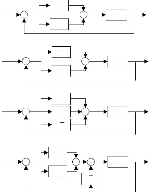
r	+	KIò0t					+	u	y
		e
							+		system
		−
		KP
(a)	PI controller
		K d
r	+	e	Ddt				+	u	y
							+		system
		−	KP
(b)	PD controller
			KP
r	+	e		t		+	+	u	y
		KIò0					+		system
		−		dtd
		K
		D
(c)	PID controller
		K ò0t
r	+	I			+		+	u	y
		e
					+				system
		−						−
		KP					d
							KDdt
(d)	PI+D controller

Figure 7 Some typical combination of P, I, D controllers.