

Chen Y.Relay feedback tuning of robust PID controllers with iso-damping property
.pdfProceedings of the 42nd IEEE |
|
Conference on Decision and Control |
WeM06-2 |
Maui, Hawaii USA, December 2003 |
Relay Feedback Tuning of Robust PID Controllers With Iso-Damping Property
YangQuan Chen, ChuanHua Hu and Kevin L. Moore
Center for Self-Organizing and Intelligent Systems (CSOIS),
Dept. of Electrical and Computer Engineering,
UMC 4160, College of Engineering, 4160 Old Main Hill,
Utah State University, Logan, UT 84322-4160, USA.
Abstract— A new tuning method for PID controller design is proposed for a class of unknown, stable, and minimum phase plants. We are able to design a PID controller to ensure that the phase Bode plot is flat, i.e., the phase derivative w.r.t. the frequency is zero, at a given frequency called the “tangent frequency” so that the closed-loop system is robus t to gain variations and the step responses exhibit an isodamping property. At the “tangent frequency”, the Nyquist curve tangentially touches the sensitivity circle. Several relay feedback tests are used to identify the plant gain and phase at the tangent frequency in an iterative way. The identified plant gain and phase at the desired tangent frequency are used to estimate the derivatives of amplitude and phase of the plant with respect to frequency at the same frequency point by Bode's integral relationship. Then, these derivatives are used to design a PID controller for slope adjustment of the Nyquist plot to achieve the robustness of the system to gain variations. No plant model is assumed during the PID controller design. Only several relay tests are needed. Simulation examples illustrate the effectiveness and the simplicity of the proposed method for robust PID controller design with an iso-damping property.
Index Terms— PID controller, PID tuning, relay feedback test, Bode's integral, flat phase condition, iso-damping propert y.
I. INTRODUCTION
According to a survey [1] of the state of process control systems in 1989 conducted by the Japan Electric Measuring Instrument Manufacturer's Association, more than 90 percent of the control loops were of the PID type. It was also indicated [2] that a typical paper mill in Canada has more than 2,000 control loops and that 97 percent use PI control. Therefore, the industrialist had concentrated on PI/PID controllers and had already developed one-button type relay auto-tuning techniques for fast, reliable PI/PID control yet with satisfactory performance [3], [4], [5], [6], [7]. Although many different methods have been proposed for tuning PID controllers, till today, the Ziegler-Nichols method [8] is still extensively used for determining the parameters of PID controllers. The design is based on the measurement of the critical gain and critical frequency of the plant and using simple formulae to compute the controller parameters. In 1984, Astr˚ ¨om and H¨agglund [9] proposed an automatic tuning method based on a simple relay feedback test which uses the describing function analysis to give the critical gain and the critical frequency of the system. This information can be used to compute a PID controller with desired gain and phase margins. In relay feedback tests, it is a common
Corresponding author: Dr YangQuan Chen. E-mail: yqchen@ece.usu.edu; Tel. +1(435)797-0148; Fax: +1(435)7973054. URL: http://www.csois.usu.edu/people/yqchen.
practice to use a relay with hysteresis [9] for noise immunity. Another commonly used technique is to introduce an artificia l time delay within the relay closed-loop system, e.g., [10], to change the oscillation frequency in relay feedback tests.
After identifying a point on the Nyquist curve of the plant, the so-called modified Ziegler-Nichols method [4], [11] can be used to move this point to another position in the complex plane. Two equations for phase and amplitude assignment can be obtained to retrieve the parameters of a PI controller. For a PID controller, however, an additional equation should be introduced. In the modified Ziegler-Nichols method, α, the ratio between the integral time Ti and the derivative time Td, is chosen to be constant, i.e., Ti = αTd, in order to obtain a unique solution.
The control performance is heavily influenced by the choice of α as observed in [10]. Recently, the role of α has drawn much attention, e.g., [12], [13], [14]. For the ZieglerNichols PID tuning method, α is generally assigned as a magic number 4 [4]. Wall´en, Astr˚ ¨om and H¨agglund proposed that the tradeoff between the practical implementation and the system performance is the major reason for choosing the ratio between Ti and Td as 4 [12].
The main contribution of this paper is the use of a new tuning rule which gives a new relationship between Ti and Td in stead of the equation Ti = 4Td proposed in the modified Ziegler-Nichols method [4], [11]. We propose to add an txtra condition that the phase Bode plot at a specified frequency wc at the point where sensitivity circle touches Nyquist curve is locally flat which implies that the system will be more robust to gain variations. This additional condition can be expressed
d6 G(s)
as ds |s=jwc = 0, which can be equivalently expressed as
6 |
dG(s) |
|s=jwc = 6 G(s)|s=jwc |
(1) |
ds |
where wc is the frequency at the point of tangency and G(s) = K(s)P (s) is the transfer function of the open loop system including the controller K(s) and the plant P (s). In this paper, we consider the PID controller of the following form:
K(s) = Kp(1 + |
1 |
+ Tds). |
(2) |
Tis |
This ”flat phase” idea proposed above is illustrated in Fig. 1(a) where the Bode diagram of the open loop system is shown with its phase being tuned locally flat around wc. We can expect that, if the gain increases or decreases a certain percentage, the phase margin will remain unchanged.
0-7803-7924-1/03/$17.00 ©2003 IEEE |
2180 |
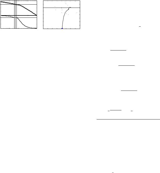
Therefore, in this case, the step responses under various gains changing around the nominal gain will exhibit an isodamping property, i.e., the overshoots of step responses will be almost the same. This can also be explained by Fig. 1(b) where the sensitivity circle touches the Nyquist curve of the open loop system at the flat phase point. Clearly, since gain variations are unavoidable in the real world due to possible sensor distortion, environment change and etc., the iso-damping is a desirable property which ensures that no harmful excessive overshoot is resulted due to gain variations.
Bode Diagram
|
50 |
|
|
|
|
|
0 |
|
|
|
|
(dB) |
|
|
|
|
|
Magnitude |
−50 |
|
|
|
|
|
|
|
|
|
|
|
−100 |
|
|
|
|
|
−150−90 |
|
|
|
|
Phase (deg) |
−180 |
|
|
|
|
−270 |
|
|
|
|
|
|
|
|
|
|
|
|
−360 |
|
|
|
|
|
10−2 |
10−1 |
100 |
101 |
102 |
|
|
|
Frequency |
(rad/sec) |
|
(a) Basic idea: a flat phase curve at gain crossover frequency
Nyquist Diagram
|
1 |
|
|
|
|
|
|
|
|
|
0.5 |
|
|
|
|
|
|
|
|
|
0 |
|
|
|
|
|
|
|
|
|
−0.5 |
|
|
|
|
|
|
|
|
Axis |
|
|
|
|
|
|
|
|
|
Imaginary |
−1 |
|
|
|
|
|
|
|
|
|
−1.5 |
|
|
|
|
|
|
|
|
|
−2 |
|
|
|
|
|
|
|
|
|
−2.5 |
|
|
|
|
|
|
|
|
|
−3 |
|
|
|
|
|
|
|
|
|
−3 |
−2.5 |
−2 |
−1.5 |
−1 |
−0.5 |
0 |
0.5 |
1 |
|
|
|
|
|
Real Axis |
|
|
|
|
(b) |
Sensitivity |
circle |
|
tangentially |
|||||
touches Nyquist curve at the flat phase
Fig. 1. Illustration of the basic idea for isodamping robust PID tuning
Assume that the phase of the open loop system at wc is
6 |
G(s)|s=jwc = Φm − π. |
(3) |
|
|
|
||
Then, the corresponding gain is |
|
||
|
|
|G(jwc )| = cos(Φm). |
(4) |
With these two conditions (3) and (4) and the new condition (1), all the three parameters of PID controller can be calculated.
As in the Ziegler-Nichols method, Ti and Td are used to tune the phase condition (3) and Kp is determined by the gain condition (4). However, the condition (1) gives a relationship between Ti and Td instead of Ti = αTd.
Note that in this new tuning method, wc is not necessarily the gain crossover frequency. wc is the frequency at which the Nyquist curve tangentially touches the sensitivity circle. Similarly, Φm, the tangent phase, is not necessarily the phase margin usually used in previous PID tuning methods. According to [4], the phase margin is always selected from 30◦ to 60◦. Due to the flat phase condition (1), the derivative of the phase near wc will be relatively small. Therefore, if Φm is selected to be around 30◦, such as 35◦, the phase margin will be generally within the desired interval.
II. SLOPE ADJUSTMENT OF THE PHASE BODE PLOT
In this section, we will show how Ti and Td are related under the new condition (1).
Substitute s by jw so that the closed loop system can be
written as G(jw) = K(jw)P (jw), where |
|
||
1 |
|
(5) |
|
K(jw) = Kp(1 + |
|
+ jwTd) |
|
jwTi |
|||
is the PID controller obtained from (2). The phase of the closed loop system is given by
6 |
G(jw) = 6 K(jw) + 6 P (jw). |
(6) |
|||||
|
|
|
|
|
|
|
|
The derivative of the closed loop system G(jw) with respect to w can be written as follows:
dG(jw) |
= P (jw) |
dK(jw) |
+ K(jw) |
dP (jw) |
. (7) |
|
dw |
dw |
dw |
||||
|
|
|
From (1), the phase of the derivative of the open loop system can not obviously be obtained directly from (7). So, we need to simplify (7).
The derivative of the controller with respect to w is |
|
|||||||||||||||||||||||||||||||||||||||
|
|
|
|
|
dK(jw) |
|
= jKp(Td + |
|
1 |
|
|
|
). |
|
|
|
(8) |
|||||||||||||||||||||||
|
|
|
|
|
|
|
|
|
|
|
|
|
|
|
|
|
|
|
||||||||||||||||||||||
|
|
|
|
|
|
dw |
|
|
|
|
|
|
|
|
|
|
|
|
|
|
|
w2Ti |
|
|
|
|||||||||||||||
To calculate dP (jw) , since we have |
|
|
|
|
|
|
|
|
|
|
|
|
|
|
|
|
|
|
|
|
||||||||||||||||||||
|
|
|
|
|
dw |
|
|
|
|
|
|
|
|
|
|
|
|
|
|
|
|
|
|
|
|
|
|
|
|
|
|
|
|
|
|
|
|
|
|
|
|
|
lnP (jw) = ln|P (jw)| + j6 |
P (jw), |
|
|
(9) |
||||||||||||||||||||||||||||||||||
differentiating (9) with respect to w gives |
|
|
|
|||||||||||||||||||||||||||||||||||||
|
|
|
|
|
dlnP (jw) |
= |
|
1 |
|
|
|
|
dP (jw) |
|
|
|
|
|||||||||||||||||||||||
|
|
|
|
|
|
|
|
dw |
P (jw) |
|
|
|
|
|
dw |
|
|
|
||||||||||||||||||||||
|
|
|
|
|
|
|
|
|
|
|
|
|
|
|
|
|
|
|||||||||||||||||||||||
|
|
|
|
|
= |
|
dln|P (jw)| |
+ j |
d6 |
P (jw) |
. |
|
|
|
(10) |
|||||||||||||||||||||||||
|
|
|
|
|
|
|
|
|
|
|
||||||||||||||||||||||||||||||
|
|
|
|
|
|
|
|
|
|
|
|
|
|
|
|
|
|
|
|
|
|
|
||||||||||||||||||
|
|
|
|
|
|
|
|
|
|
dw |
|
|
|
|
|
|
|
|
|
|
dw |
|
|
|
||||||||||||||||
Straightforwardly, we arrive at |
|
|
|
|
|
|
|
|
|
|
|
|
|
|
|
|
|
|
|
|
||||||||||||||||||||
|
dP (jw) |
|
= P (jw)[ |
dln|P (jw)| |
|
+ j |
d6 |
P (jw) |
]. |
|
(11) |
|||||||||||||||||||||||||||||
|
|
|
|
|
|
|
|
|
|
|||||||||||||||||||||||||||||||
|
dw |
|
dw |
|
|
|
|
|
|
|||||||||||||||||||||||||||||||
|
|
|
|
|
|
|
|
|
|
|
|
|
|
|
|
|
|
|
|
|
|
|
dw |
|
|
|
||||||||||||||
Substituting (5), (8) and (11) into (7) gives |
|
|
|
|||||||||||||||||||||||||||||||||||||
|
|
dG(jw) |
|
|
|
|
|
|
|
|
|
|
|
|
|
|
1 |
|
|
|
|
|||||||||||||||||||
|
|
|
|
|
|
|
|
|
= KpP (jw)[j(Td + |
|
|
|
) |
|
|
|
||||||||||||||||||||||||
|
|
|
|
dw |
|
|
|
|
w2Ti |
|
|
|
||||||||||||||||||||||||||||
+(1 + j(T |
w |
|
|
|
1 |
))( |
dln|P (jw)| |
|
d6 |
P (jw) |
)]. |
(12) |
||||||||||||||||||||||||||||
|
|
|
|
+ j |
|
|
||||||||||||||||||||||||||||||||||
|
|
|
|
|
|
|
|
|||||||||||||||||||||||||||||||||
|
|
d |
|
− wTi |
|
|
|
dw |
|
|
|
|
|
|
|
|
|
|
|
|
|
|
|
dw |
|
|
|
|||||||||||||
Hence, the slope of the Nyquist curve at any specific frequency w0 is given by
6 |
dG(jw) |
|w0 = 6 P (jw0)+ |
dw |
(Td Ti w2 + 1) + (Td Tiw2 − 1)sa (w0) + sp (w0)Ti w0
tan−1[ 0 0 ] (13) sa(w0)Ti w0 − (Td Tiw02 − 1)sp (w0)
where, following the notations introduced in [15], [16], sa(w0) and sp (w0) are used throughout this paper defined as follows:
s |
(w ) = w |
|
dln|P (jw)| |
|w |
0 , |
(14) |
||||
a |
0 |
0 |
|
|
|
dw |
|
|
|
|
sp(w0) = w0 |
d6 |
P (jw) |
|w0 . |
(15) |
||||||
|
|
|
||||||||
|
|
dw |
||||||||
Here, our task is to adjust the slope of the Nyquist curve to match the condition shown in (1). By combining (1), (6) and (13), one obtains
6 K(jw)|w0 = tan−1[
2181

(TdTiw02 + 1) + (TdTiw02 − 1)sa(w0) + sp(w0)Tiw0 |
]. |
|
sa(w0)Tiw0 − (TdTiw02 − 1)sp(w0) |
||
(16) |
After a straightforward calculation, one obtains the relation-
ship between Ti and Td as follows: |
|
|||
|
√ |
|
|
|
Td = |
−Tiw0 + 2sp(w0) + |
, |
(17) |
|
|
2sp(w0)w2Ti |
|
||
|
0 |
|
|
|
where = Ti2w02 −8sp(w0)Tiw0 −4Ti2w02s2p(w0). Note that due to the nature of the quadratic equation, an alternative
relationship, i.e., has been discarded.
The approximation of sp for stable and minimum phase
plant can be given as follows [17]: |
|
|
||||||
|
sp(w0) = w0 |
d6 |
P (jw) |
|w0 |
|
|||
|
|
|
|
|
||||
|
dw |
|
||||||
2 |
|
|
|
|
|
(18) |
||
≈ 6 |
P (jw0) + |
|
[ln|Kg | − ln|P (jw0)|] |
|||||
π |
||||||||
where |Kg | = P (0) is the static gain of the plant, 6
is the phase and |P (jw0)| is the gain of the plant at the specific frequency w0.
It is obvious that Ti and Td are related by sp alone. For this new tuning method, sp includes all the information that we need of the unknown plant. In what follows, we show that the sp estimate formula can be extended to plants with integrators and/or time delay.
Consider the plant with m integrators |
|
||
|
˜ |
|
|
P (s) = |
P (s) |
, m = 1, 2, 3, · · · . |
(19) |
sm |
|||
Clearly, one can not get the static gain of such systems to compute sp directly. But from (15),
d6 P (jw)
sp(w0) = w0 dw |w0
6 |
˜ |
mπ |
|
6 |
˜ |
|
|
||||
|
d( |
|
P (jw) − |
2 |
) |
|
d |
|
P (jw) |
|
(20) |
|
|
|
|
||||||||
= w0 |
dw |
|
|
|w0 = w0 |
dw |
|w0 , |
|||||
|
|
|
|||||||||
which means that for the systems with integrators, sp should be estimated according to the systems without any integrator.
For the plant with a time delay τ
|
|
|
|
|
|
|
|
˜ |
¯ |
|
|
−τ s |
, |
|
(21) |
|||||||
|
|
|
|
|
|
|
|
P (s) = P (s)e |
|
|
|
|
||||||||||
in the same way, |
|
|
|
|
|
|
|
|
|
|
|
|
|
|||||||||
sp(w0) = w0 |
|
d6 |
P˜(jw) |
|w0 = w0 |
|
d6 P¯(jw) |
|w0 − τ w0 |
. (22) |
||||||||||||||
|
|
|
|
|
|
|
|
|
|
|
||||||||||||
|
|
|
|
dw |
|
|
|
|
dw |
|||||||||||||
Consequently, substituting (18), we obtain |
|
|
||||||||||||||||||||
|
6 |
¯ |
|
|
2 |
|
|
|
|
|
|
¯ |
|
|
||||||||
|
|
|
|
|
|
|
|
|
|
|
|
|
|
|
||||||||
sp (w0) ≈ |
|
|
|
|
|
P (jw0) + π [ln|Kg | − ln|P (jw0)|] − τ w0 |
||||||||||||||||
|
6 |
|
|
˜ |
2 |
|
|
|
|
|
|
|
˜ |
|
(23) |
|||||||
|
|
|
|
|
|
|
|
|
|
|
|
|
|
|||||||||
≈ |
|
|
|
P (jw0) + |
|
π [ln|Kg |
| − ln|P (jw0)|]. |
|||||||||||||||
Obviously, the time delay will not contribute to the estimation of sp .
So, in general, for the plant with both integrators and a time delay
|
|
|
˜ |
|
|
|
¯ |
|
|
−τ s |
|
|
||||||||
P (s) = |
P (s) |
|
= |
|
P (s)e |
|
|
, m = 1, 2, 3, · · · , |
(24) |
|||||||||||
sm |
|
|
|
sm |
|
|||||||||||||||
according to (20) and (23), |
|
|
|
|
|
|
|
|
|
|||||||||||
sp(w0) = w0 |
|
d6 |
P (jw) |
|w0 = w0 |
d6 |
P˜(jw) |
|w0 |
|
||||||||||||
|
|
|
|
|
|
|
|
|
|
|
|
|||||||||
|
|
|
|
dw |
|
|
dw |
|
||||||||||||
|
6 |
˜ |
|
|
|
|
|
2 |
|
|
|
|
˜ |
|
(25) |
|||||
|
|
|
|
|
|
|
|
|
|
|
|
|||||||||
≈ |
|
|
P (jw0) + |
π [ln|Kg | − ln|P (jw0)|]. |
|
|||||||||||||||
III. THE NEW PID CONTROLLER DESIGN FORMULAE
Suppose that we have known sp at wc. How to experimentally measure sp(wc ) will be discussed in the next section based on the measurement of 6 P (jwc) and |P (jwc )|.
To write down explicitly the formulae for Kp, Ti and Td, let us summarize what are known at this point. We are given i) wc , the desired tangent frequency; ii) Φm, the desired tangent phase; iii) measurement of 6 P (jwc) and |P (jwc )| and iv) the estimation of sp(wc ).
Furthermore, using (3) and (4), the PID controller param-
eters can be set as follows: |
|
|
|
|
|
||||
Kp = |
|
|
cos(Φm) |
, |
(26) |
||||
|
|
|
|||||||
|P (jwc)p |
1 + tan2(Φm − 6 |
P (jwc )) |
| |
||||||
|
|
|
|||||||
Ti = |
|
|
−2 |
, |
(27) |
||||
|
ˆ |
2 ˆ |
|||||||
|
|
|
|
|
|||||
|
|
wc[sp(wc ) + Φ) + tan (Φ)sp(wc )] |
|
|
|||||
where ˆ m 6 c .Finally, d can be computed from
Φ = Φ − P (jw ) T
(17).
Remark 3.1: The selection of wc heavily depends on the system dynamics. For most of plants, there exists an interval for the selection of wc to achieve flat phase condition. If no better idea about wc, the desired cutoff frequency can used
as the initial value. For Φm, a good choice is within 30◦ to 35◦.
IV. MEASURING arg P (jwc) , |P (jwc)| AND sp (wc) VIA
RELAY FEEDBACK TESTS
Following the discussion in the above section, the parameters of a PID controller can be calculated straightforwardly if we know 6 P (jwc), |P (jwc )| and sp(wc ).
As indicated in (18), sp(wc) can be obtained from the knowledge of the static gain |P (0)|, 6 P (jwc ) and |P (jwc)|. The static gain |P (0)| or Kg is very easy to measure and it is assumed to be known. The relay feedback test, shown in Fig. 2, can be used to “measure” 6 P (jwc ) and |P (jwc)|. In the relay feedback experiments, a relay is connected in closed-loop with the unknown plant as shown in Fig. 2 which is usually used to identify one point on the Nyquist diagram of the plant. To change the oscillation frequency due to relay feedback, an artificial time delay is introduced in the loop. The artificial time delay θ is the tuning knob here to change the oscillation frequency. Our problem here is how to get the right value of θ which corresponds to the tangent frequency wc. To solve this problem, an iterative method can be used as summarized in the following:
2182
|
|
|
|
|
|
|
|
|
|
|
|
|
|
|
|
|
|
|
|
|
|
|
The PID controller designed by the modified Ziegler-Nichols |
||||||||||||||||||
|
|
|
|
|
|
|
|
|
|
|
|
|
|
|
|
|
|
|
|
|
|
|
method is |
|
|
|
|
|
|
|
|
|
|
|
|
|
|
|
|
||
|
|
|
|
|
|
|
|
|
|
|
|
|
|
|
|
|
|
|
|
|
|
|
|
K1(s) = 1.131(1 + |
|
|
1 |
+ 0.781s). |
|
(33) |
|||||||||||
|
Fig. 2. |
Relay plus artificial time delay ( θ) feedback system |
|
3.124s |
|
||||||||||||||||||||||||||||||||||||
1) |
Start with the desired tangent frequency wc. |
|
|
|
|
Bode Diagram |
|
|
|
|
|
|
|
|
Nyquist Diagram |
|
|
|
|
||||||||||||||||||||||
|
|
50 |
|
|
|
|
|
|
|
1 |
|
|
|
|
|
|
|
|
|
||||||||||||||||||||||
2) |
Select two different values (θ−1 |
and θ0) for the time |
0 |
|
|
|
|
|
|
|
0.5 |
|
|
|
|
|
|
|
|
|
|||||||||||||||||||||
|
delay parameter properly and do the relay feedback test |
Magnitude(dB) |
|
|
|
|
|
|
|
0 |
|
|
|
|
|
|
|
|
|
||||||||||||||||||||||
|
|
|
|
|
|
|
|
|
|
|
|
|
|
|
|
|
|
|
|
|
|
|
−50 |
|
|
|
|
|
|
|
|
|
|
|
|
|
|
|
|
|
|
|
twice. Then, two points on the Nyquist curve of the |
−100 |
|
|
|
|
|
|
Axis |
−0.5 |
|
|
|
|
|
|
|
|
|
||||||||||||||||||||||
|
|
|
|
|
|
|
|
|
|
|
|
|
|
|
|
|
|||||||||||||||||||||||||
|
plant can be obtained. The frequencies of these points |
−150−90 |
|
|
|
|
|
|
Imaginary |
−1 |
|
|
|
|
|
|
|
|
|
||||||||||||||||||||||
|
|
|
|
|
|
|
|
|
|
|
|
|
|
|
|
|
|
||||||||||||||||||||||||
|
can be represented as w−1 |
|
and w0 |
which correspond |
(deg) |
|
|
|
|
|
|
|
−1.5 |
|
|
|
|
|
|
|
|
|
|||||||||||||||||||
|
|
|
|
|
|
|
|
|
−2 |
|
|
|
|
|
|
|
|
|
|||||||||||||||||||||||
|
|
|
|
|
|
|
|
|
|
|
|
|
|
|
|
|
|
|
|
|
|
|
−180 |
|
|
|
|
|
|
|
|
|
|
|
|
|
|
|
|
|
|
|
to θ−1 and θ0, respectively. The iteration begins with |
Phase |
|
|
|
|
|
|
|
−2.5 |
|
|
|
|
|
|
|
|
|
||||||||||||||||||||||
|
−270 |
|
|
|
|
|
|
|
|
|
|
|
|
|
|
|
|
||||||||||||||||||||||||
|
these initial values (θ |
−1 |
, w |
|
|
|
) and (θ |
0 |
, w ). |
|
|
−360 −2 |
−1 |
0 |
1 |
|
|
2 |
|
−3 |
−2.5 |
−2 |
−1.5 |
−1 |
−0.5 |
0 |
0.5 |
1 |
|||||||||||||
3) |
|
|
|
|
|
−1 |
|
|
|
|
|
|
|
0 |
|
|
|
10 |
10 |
10 |
10 |
|
|
10 |
|
−3 |
|||||||||||||||
With the values obtained in the previous iterations, the |
|
|
Frequency |
(rad/sec) |
|
|
|
|
|
|
|
|
Real Axis |
|
|
|
|
||||||||||||||||||||||||
|
artificial time delay parameter |
|
θ can be updated using |
(a) Comparison of Bode plots |
|
|
(b) Comparison of Nyquist plots |
||||||||||||||||||||||||||||||||||
|
|
|
|
|
|
|
|
|
|
|
|
|
|
|
|
|
|
|
|
||||||||||||||||||||||
|
a simple interpolation/extrapolation scheme as follows: |
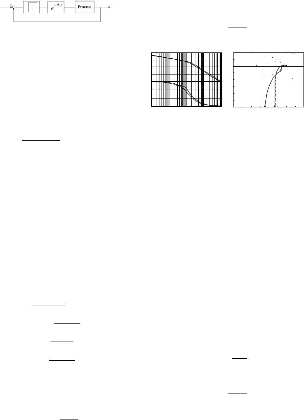
Fig. 3. Frequency responses of K1p (s)P2(s) and K1(s)P2(s) (Dashed |
|||||||||||||||||||||||||||||||||||||||
|
|
|
|
|
|
|
|
|
|
|
|
|
|
|
|
|
|
|
|
|
|
|
|||||||||||||||||||
|
θ |
|
= |
wc − wn−1 |
(θ |
n−1 − |
θ |
|
|
|
) + θ |
|
|
line: The modified Ziegler-Nichols, Solid line: The propose d) |
|
|
|
|
|||||||||||||||||||||||
|
n |
n−2 |
n−1 |
|
|
|
|
|
|
|
|
|
|
|
|
|
|
|
|
|
|
||||||||||||||||||||
|
|
|
wn−1 − wn−2 |
|
|
|
|
The Bode and the Nyquist plots are compared in Fig. 3. |
|||||||||||||||||||||||||||||||||
|
where n represents the current iteration number. With |
From the Bode plots, it is seen that the phase curve near the |
|||||||||||||||||||||||||||||||||||||||
|
the new θn, after the relay test, the corresponding |
frequency wc=0.4 rad./s is flat. The phase margin roughly |
|||||||||||||||||||||||||||||||||||||||
|
frequency wn can be recorded. |
|
|
|
|
|
|
|
|
|
|
equals |
45◦. That means |
the controller moves the point |
|||||||||||||||||||||||||||
4) |
Compare wn with wc. If |
wn |
− |
w |
| |
< δ, quit iteration. |
P (0.4j) of the Nyquist |
curve to |
K(0.4j)P (0.4j) |
on the unit |
|||||||||||||||||||||||||||||||
|
|
|
|
|
|
|
| |
|
|
|
|
|
|
|
|
|
|
|
|
◦ |
|
|
|
|
|
|
|||||||||||||||
|
Otherwise, go to Step 3. Here, δ is a small positive |
circle with a phase of 135 |
|
and at the same time makes the |
|||||||||||||||||||||||||||||||||||||
|
number. |
|
|
|
|
|
|
|
|
|
|
|
|
|
|
|
|
|
|
|
|
Nyquist curve satisfy (1). |
|
|
|
|
|
|
|
|
|
|
|
|
|
||||||
The iterative method proposed above is feasible because |
However, in Fig. 3(b), the Nyquist plot of the open |
||||||||||||||||||||||||||||||||||||||||
in general the relationship between the delay time θ and the |
loop system is not tangential to the sensitivity |
circle |
at |
||||||||||||||||||||||||||||||||||||||
oscillation frequency w is one-to-one. |
|
|
|
|
|
|
|
|
|
the flat phase but to another point on the Nyquist curve. |
|||||||||||||||||||||||||||||||
After the iteration, the final oscillation frequency is quit e |
Define [wl , wh] |
the frequency interval corresponding to the |
|||||||||||||||||||||||||||||||||||||||
close to the desired one wc so that the oscillation frequency |
flat phase. So, the gain crossover frequency |
wc |
can |
be |
|||||||||||||||||||||||||||||||||||||
is considered as wc. Hence, the amplitude and the phase of |
moved within [wl , wh] by adjusting |
Kp |
by |
Kp0 |
= |
βKp |
|||||||||||||||||||||||||||||||||||
the plant at the specified frequency can be obtained. Using |
|
|
wl |
wh |
|
|
|
|
|
|
|
|
|
|
|
|
|
|
|||||||||||||||||||||||
where0 |
β [ wc , wc ]. For this |
example, if Kp is |
changed |
||||||||||||||||||||||||||||||||||||||
(18), one can calculate the approximation of sp. |
|
|
|
||||||||||||||||||||||||||||||||||||||
|
|
|
to Kp |
= 0.7Kp = 0.652, |
the flat phase segment will |
||||||||||||||||||||||||||||||||||||
|
|
|
|
|
|
|
|
|
|
|
|
|
|
|
|
|
|
|
|
|
|
|
tangentially touch the sensitivity circle. The Nyquist plot |
||||||||||||||||||
|
|
|
V. ILLUSTRATIVE EXAMPLES |
|
|
|
|
of the open loop system with the modified proposed PID |
|||||||||||||||||||||||||||||||||
|
|
|
|
|
|
|
controller, |
i.e., |
0.7C1p(s), |
is |
shown |
in Fig. |
4(a) |
and |
the |
||||||||||||||||||||||||||
The new |
PID |
design method |
|
|
presented |
above |
will be |
||||||||||||||||||||||||||||||||||
|
|
step responses |
of the |
closed |
|
loop system |
are |
compared |
|||||||||||||||||||||||||||||||||
illustrated via some simulation examples. In the simulation, |
|
||||||||||||||||||||||||||||||||||||||||
in Fig. 4(b). Comparing |
the |
closed-loop |
system |
with |
the |
||||||||||||||||||||||||||||||||||||
the following classes of plants, studied in [12], will be used. |
|||||||||||||||||||||||||||||||||||||||||
modified proposed PID controller to that with the modi- |
|||||||||||||||||||||||||||||||||||||||||
|
|
|
|
|
|
|
|
|
|
|
|
|
|
|
|
|
|
|
|
|
|
|
|||||||||||||||||||
|
|
|
|
1 |
|
|
|
|
|
|
|
|
|
|
|
|
|
|
|
|
(28) |
fied Ziegler-Nichols controller, the overshoots of the step |
|||||||||||||||||||
|
Pn (s) = (s + 1)(n+3) |
, n = 1, 2, 3, 4; |
|
|
responses from the proposed scheme remain almost invariant |
||||||||||||||||||||||||||||||||||||
|
|
|
|
|
|
|
|
1 |
|
|
|
|
|
|
|
|
|
|
|
|
under |
gain |
variations. However, |
the |
overshoots |
using |
the |
||||||||||||||
|
|
|
|
P5(s) = |
|
|
|
|
|
; |
|
|
|
|
|
|
|
(29) |
modified Ziegler-Nichols controller change remarkably. |
|
|
||||||||||||||||||||
|
|
|
|
|
|
|
|
|
|
|
3 |
|
|
|
|
|
|
|
|
|
|||||||||||||||||||||
|
|
|
|
|
s(s + 1) |
|
|
|
|
|
|
|
|
|
B. Plant with an Integrator P5(s) |
|
|
|
|
|
|
|
|
||||||||||||||||||
|
|
|
|
|
|
|
1 |
|
|
|
3 e−s; |
|
|
|
|
|
|
(30) |
|
|
|
|
|
|
|
|
|||||||||||||||
|
|
|
|
P6(s) = |
|
|
|
|
|
|
|
|
|
|
|
For the plant P5(s), the proposed controller is |
|
|
|
|
|||||||||||||||||||||
|
|
|
|
|
|
|
|
|
|
|
|
|
|
|
|
|
|
|
|
||||||||||||||||||||||
|
|
|
|
|
(s + 1) |
|
|
|
|
|
|
|
|
|
|
|
|
|
|
|
|
|
|
|
|
|
|
|
|
|
|
|
|
|
|||||||
|
|
|
|
|
|
|
1 |
|
|
|
|
|
|
|
|
|
|
|
|
|
|
|
|
|
|
|
|
|
|
|
|
1 |
|
|
|
|
|
|
|
|
|
|
|
|
|
P7(s) = |
|
|
|
|
|
|
3 e−s; |
|
|
|
|
|
|
(31) |
|
|
K2p(s) = 0.33(1 + 6.53s + 1.89s) |
|
|
|
|
||||||||||||||||
|
|
|
|
s(s + 1) |
|
|
|
|
|
|
|
|
|
|
|
|
|||||||||||||||||||||||||
|
|
|
|
|
|
|
|
|
|
|
|
|
|
|
|
with respect to β=1, wc=0.4 rad/s and Φm=45◦. The con- |
|||||||||||||||||||||||||
A. High-order Plant P2(s) |
|
|
|
|
|
|
|
|
|
|
|
|
|
|
|
|
|
||||||||||||||||||||||||
|
|
|
|
|
|
|
|
|
|
|
|
|
|
|
|
|
troller designed by the modified Ziegler-Nichols method is |
||||||||||||||||||||||||
Consider plant P2(s) in (28). This plant was also used |
|||||||||||||||||||||||||||||||||||||||||
|
|
|
|
|
|
|
|
|
1 |
|
|
|
|
|
|
|
|
||||||||||||||||||||||||
in [15]. The specifications are set as |
|
wc=0.4 |
rad./s. and |
|
K2(s) = 0.528(1 + |
|
|
+ 1.799s). |
|
|
|
||||||||||||||||||||||||||||||
Φm =45◦. The PID controller designed by using the pro- |
|
7.195s |
|
|
|
||||||||||||||||||||||||||||||||||||
posed tuning formulae is |
|
|
|
|
|
|
|
|
|
|
|
|
|
|
|
|
|
|
The Bode plot of this situation, shown in Fig. 5(a), is |
||||||||||||||||||||||
|
K1p(s) = 0.921(1 + |
|
|
1 |
|
|
+ 1.969s). |
|
(32) |
quite different with that of plant P2(s). The flat phase occurs |
|||||||||||||||||||||||||||||||
|
1.961s |
|
at the peak of the phase Bode plot. The Nyquist diagrams |
||||||||||||||||||||||||||||||||||||||
|
|
|
|
|
|
|
|
|
|
|
|
|
|
|
|
|
|
|
|
|
|
|
|
|
|
|
|
|
|
|
|
|
|
||||||||
2183
1
0.5
0 


−0.5
−1
−1.5
−2
−2.5
−3 |
|
|
|
|
|
|
|
|
−3 |
−2.5 |
−2 |
−1.5 |
−1 |
−0.5 |
0 |
0.5 |
1 |
(a) Comparison of Nyquist plots
Step Response
1.4 |
|
|
|
|
|
|
|
|
1.2 |
|
|
|
|
|
|
|
|
1 |
|
|
|
|
|
|
|
|
0.8 |
|
|
|
|
|
|
|
|
Amplitude |
|
|
|
|
|
|
|
|
0.6 |
|
|
|
|
|
|
|
|
0.4 |
|
|
|
|
|
|
|
|
0.2 |
|
|
|
|
|
|
|
|
0 |
|
|
|
|
|
|
|
|
0 |
10 |
20 |
30 |
40 |
50 |
60 |
70 |
80 |
Time (sec)
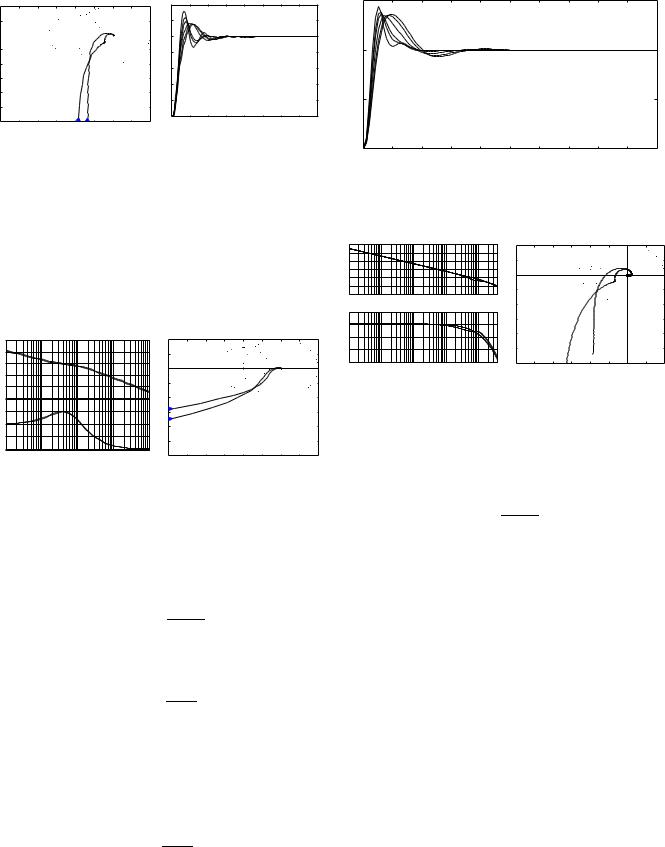
(b) Comparison of step responses
Fig. 4. Comparisons of frequency responses and step responses of
0.7K1p (s)P2(s) and K1(s)P2(s) (Dashed line: The modified ZieglerNichols, Solid line: The proposed. For both schemes, gain variations 1,
1.1, 1.3 are considered in step responses)
are compared in Fig. 5(b). The step responses are compared in Fig. 6 where the proposed controller does not exhibit an obviously better performance than the modified ZieglerNichols controller for the iso-damping property because of the effect of the integrator.
Bode Diagram
|
100 |
|
|
|
|
|
50 |
|
|
|
|
(dB) |
0 |
|
|
|
|
Magnitude |
−50 |
|
|
|
|
|
|
|
|
|
|
|
−100 |
|
|
|
|
|
−150−90 |
|
|
|
|
|
−135 |
|
|
|
|
(deg) |
−180 |
|
|
|
|
Phase |
|
|
|
|
|
|
|
|
|
|
|
|
−225 |
|
|
|
|
|
−270 |
|
|
|
|
|
10−2 |
10−1 |
100 |
101 |
102 |
|
|
|
Frequency |
(rad/sec) |
|
(a) Comparison of Bode plots
1 |
|
|
|
|
|
|
|
|
0.5 |
|
|
|
|
|
|
|
|
0 |
|
|
|
|
|
|
|
|
−0.5 |
|
|
|
|
|
|
|
|
−1 |
|
|
|
|
|
|
|
|
−1.5 |
|
|
|
|
|
|
|
|
−2 |
|
|
|
|
|
|
|
|
−2.5 |
|
|
|
|
|
|
|
|
−3 |
|
|
|
|
|
|
|
|
−3 |
−2.5 |
−2 |
−1.5 |
−1 |
−0.5 |
0 |
0.5 |
1 |
(b) Comparison of Nyquist plots
Fig. 5. Comparisons of frequency responses of K2p (s)P5(s) and K2(s)P5(s) (Dashed line: The modified Ziegler-Nichols, Solid line: The proposed)
C. Plant with a Time Delay P6(s)
For the plant P6(s) the proposed controller is
1
K3p(s) = 1.024(1 + 1.241s + 1.539s)
with respect to β=0.7, wc=0.6 rad/s and Φm=30◦. The controller designed by the modified Ziegler-Nichols method is
1
K3(s) = 1.674(1 + 2.57s + 0.643s).
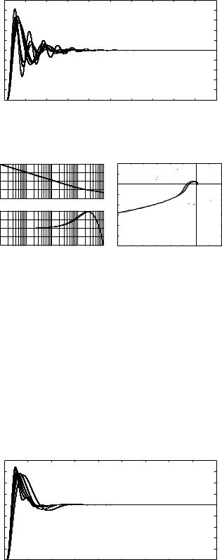
The Bode plots and Nyquist plots are compared Fig. 7. The step responses are compared in Fig. 8 where the iso-damping property can be clearly observed.
D. Plant with an Integrator and a Time Delay P7(s)
For the plant P7(s), the proposed controller is
1
K4p = 0.212(1 + 9.52s + 2.061s)
Step Response
1.5 |
|
|
|
|
|
|
|
|
|
|
1 |
|
|
|
|
|
|
|
|
|
|
Amplitude |
|
|
|
|
|
|
|
|
|
|
0.5 |
|
|
|
|
|
|
|
|
|
|
0 |
|
|
|
|
|
|
|
|
|
|
0 |
10 |
20 |
30 |
40 |
50 |
60 |
70 |
80 |
90 |
100 |
Time (sec)
Fig. 6. Comparison of step responses of K2p (s)P5(s) and K2(s)P5(s) (Solid line: The proposed modified controller with gain vari ations 1, 0.9, 0.8; Dotted line: The modified Ziegler-Nichols controller with g ain variations 1, 0.9, 0.8)
200 |
|
|
|
|
|
|
|
|
1 |
|
|
|
|
|
|
|
|
150 |
|
|
|
|
|
|
|
|
|
|
|
|
|
|
|
|
|
100 |
|
|
|
|
|
|
|
|
0.5 |
|
|
|
|
|
|
|
|
50 |
|
|
|
|
|
|
|
|
|
|
|
|
|
|
|
|
|
0 |
|
|
|
|
|
|
|
|
0 |
|
|
|
|
|
|
|
|
|
|
|
|
|
|
|
|
|
|
|
|
|
|
|
|
|
|
−50 |
|
|
|
|
|
|
|
|
|
|
|
|
|
|
|
|
|
|
|
|
|
|
|
|
|
|
−0.5 |
|
|
|
|
|
|
|
|
−100 |
10−3 |
10−2 |
10−1 |
100 |
|
|
|
|
|
|
|
|
|
||||
|
|
|
|
|
|
|
|
|
|
||||||||
|
|
|
|
|
|
|
|
|
−1 |
|
|
|
|
|
|
|
|
0 |
|
|
|
|
|
|
|
|
|
|
|
|
|
|
|
|
|
|
|
|
|
|
|
|
|
|
−1.5 |
|
|
|
|
|
|
|
|
−100 |
|
|
|
|
|
|
|
|
|
|
|
|
|
|
|
|
|
−200 |
|
|
|
|
|
|
|
|
−2 |
|
|
|
|
|
|
|
|
|
|
|
|
|
|
|
|
|
|
|
|
|
|
|
|
|
|
−300 |
|
|
|
|
|
|
|
|
−2.5 |
|
|
|
|
|
|
|
|
−400 |
10 |
−3 |
10 |
−2 |
10 |
−1 |
10 |
0 |
−3 |
−2.5 |
−2 |
−1.5 |
−1 |
−0.5 |
0 |
0.5 |
1 |
|
|
|
|
|
−3 |
||||||||||||
(a) Comparison of Bode plots |
(b) Comparison of Nyquist plots |
|
Fig. 7. |
Comparisons of frequency |
responses of K3p (s)P6(s) and |
K3(s)P6(s) (Dashed line: The modified Ziegler-Nichols, Solid line: The proposed)
with respect to β=1, wc=0.25 rad/s and Φm=39◦. The controller designed by the modified Ziegler-Nichols method is
1
K4 = 0.273(1 + 2.161s + 8.644s).
The Bode plots and Nyquist plots are compared Fig. 9. The step responses are compared in Fig. 10 where the isodamping property can be clearly observed.
VI. CONCLUSIONS
A new PID tuning method is proposed for a class of unknown, stable and minimum phase plants. Given the tangent frequency wc, the tangent phase Φm and with an additional condition that the phase Bode plot at wc is locally flat, we can design the PID controller to ensure that the closed loop system is robust to gain variations and to ensure that the step responses exhibit an iso-damping property. No plant model is assumed during the PID controller design. Only several relay tests are needed. Simulation examples illustrate the effectiveness and the simplicity of the proposed method for robust PID controller design with an iso-damping property for different types of plants.
Our further research efforts include 1) determining the width and the position of the flat phase so as to achieve the performance of the proposed controller and simplify the design procedure; 2) testing on more types of plants; 3) exploring nonminimum phase, open loop unstable systems.
2184
2
1.8
1.6
1.4
1.2
1
0.8
0.6
0.4
0.2
0 
0 |
10 |
20 |
30 |
40 |
50 |
60 |
70 |
80 |
90 |
100 |
Fig. 8. Comparison of step responses of K3p (s)P6(s) and K3(s)P6(s) (Solid line: The proposed modified controller with gain vari ations 1, 1.5, 1.7; Dotted line: The modified Ziegler-Nichols controller with g ain variations 1, 1.5, 1.7)
300 |
|
|
|
|
|
1 |
|
|
|
|
|
|
|
|
200 |
|
|
|
|
|
0.5 |
|
|
|
|
|
|
|
|
100 |
|
|
|
|
|
|
|
|
|
|
|
|
|
|
|
|
|
|
|
|
0 |
|
|
|
|
|
|
|
|
0 |
|
|
|
|
|
|
|
|
|
|
|
|
|
|
|
|
|
|
|
|
−0.5 |
|
|
|
|
|
|
|
|
−100 |
10−3 |
10−2 |
10−1 |
100 |
|
|
|
|
|
|
|
|
|
|
|
|
|
|
|
|
|
|
|
|
|||||
|
|
|
|
|
|
−1 |
|
|
|
|
|
|
|
|
−140 |
|
|
|
|
|
|
|
|
|
|
|
|
|
|
|
|
|
|
|
|
−1.5 |
|
|
|
|
|
|
|
|
−160 |
|
|
|
|
|
|
|
|
|
|
|
|
|
|
|
|
|
|
|
|
−2 |
|
|
|
|
|
|
|
|
−180 |
|
|
|
|
|
|
|
|
|
|
|
|
|
|
−200 |
|
|
|
|
|
−2.5 |
|
|
|
|
|
|
|
|
|
|
|
|
|
|
|
|
|
|
|
|
|
|
|
−220 |
−3 |
−2 |
−1 |
10 |
0 |
−3 |
−2.5 |
−2 |
−1.5 |
−1 |
−0.5 |
0 |
0.5 |
1 |
|
10 |
10 |
10 |
|
−3 |
|||||||||
(a) Comparison of Bode plots |
(b) Comparison of Nyquist plots |
|
Fig. 9. |
Comparisons of frequency |
responses of K4p (s)P7(s) and |
K4(s)P7(s) (Dashed line: The modified Ziegler-Nichols, Solid line: The proposed)
ACKNOWLEDGEMENT
The first author is grateful to Professor Li-Chen Fu, Editor- in-Chief of
Asian Journal of Control for providing a complimentary copy of the “Special
Issue on Advances in PID Control”, Asian J. of Control (vol. 4, no. 4). We
also thank Professor Blas M. Vinagre's comments on an early version of
this paper.
VII. REFERENCES
[1]S. Yamamoto and I. Hashimoto, “Recent status and future needs: The view from Japanese industry,” in
Proceedings of the fourth International Conference on
1.8
1.6
1.4
1.2
1
0.8
0.6
0.4
0.2
0 
0 |
20 |
40 |
60 |
80 |
100 |
120 |
140 |
160 |
180 |
Fig. 10. Comparison of step responses of K4p (s)P7(s) and K4(s)P7(s) (Solid line: The proposed modified controller with gain vari ations 1, 1.5, 1.7; Dotted line: The modified Ziegler-Nichols controller with g ain variations 1, 1.5, 1.7)
Chemical Process Control, Arkun and Ray, Eds., Texas, 1991, Chemical Process Control – CPCIV.
[2]W. L. Bialkowski, “Dreams versus reality: A view from both sides of the gap,” Pulp and Paper Canada, vol. 11, pp. 19–27, 1994.
[3]A. Leva, “PID autotuning algorithm based on relay
feedback,” IEEE Proc. Part-D, vol. 140, no. 5, pp. 328–338, 1993.
[4] Tore Hagglund Karl J. Astrom, PID Controllers: Theory, Design, and Tuning, ISA - The Instrumentation, Systems, and Automation Society (2nd edition), 1995.
[5]Cheng-Ching Yu, Autotuning of PID Controllers: Relay Feedback Approach, Advances in Industrial Control. Springer-Verlag, London, 1999.
[6]Kok Kiong Tan, Wang Qing-Guo, Hang Chang Chieh, and Tore Hagglund, Advances in PID Controllers, Advances in Industrial Control. Springer-Verlag, London, 2000.
[7]Shankar P. Bhattacharyya Aniruddha Datta, MingTzu Ho, Structure and Synthesis of PID Controllers, Springer-Verlag, London, 2000.
[8]J. G. Ziegler and N. B. Nichols, “Optimum settings for automatic controllers,” Trans. ASME, vol. 64, pp.
759–768, 1942.
[9] K. J. Astr˚ ¨om and T. H¨agglund, “Automatic tuning of simple regulators with specifications on phase and amplitude margins,” Automatica, vol. 20, no. 5, pp. 645–651, 1984.
[10]K. K. Tan, T. H. Lee, and Q. G. Wang, “Enhanced automatic tuning procedure for process control of PI/PID controllers,” AlChE Journal, vol. 42, no. 9, pp. 2555– 2562, 1996.
[11]C. C. Hang, K. J. Astr˚ ¨om, and W. K. Ho, “Refinements of the Ziegler-Nichols tuning formula,” IEE Proc. Pt. D, vol. 138, no. 2, pp. 111–118, 1991.
[12]A. Wall´en, K. J. Astr˚ ¨om, and T. H¨agglund, “Loopshaping design of PID controllers with constant ti/td ratio,” Asian Journal of Control, vol. 4, no. 4, pp. 403– 409, 2002.
[13]H. Panagopoulos, K. J. Astr˚ ¨om, and T. H¨agglund, “Design of PID controllers based on constrained optimization,” in Proceedings of the American Control Conference, San Diego, CA, 1999.
[14]B. Kristiansson and B. Lennartsson, “Optimal PID controllers including roll off and Schmidt predictor structure,” in Proceedings of IFAC 14th World Congress, Beijing, P. R. China, 1999, vol. F, pp. 297–302.
[15]A. Karimi, D. Garcia, and R. Longchamp, “PID controller design using Bode's integrals,” in Proceedings of the American Control Conference, Anchorage, AK, 2002, pp. 5007–5012.
[16]A. Karimi, D. Garcia, and R. Longchamp, “Iterative controller tuning using Bode's integrals,” in Proceedings of the 41st IEEE Conference on Decision and Control, Las Vegas, Nevada, 2002, pp. 4227–4232.
[17]H. W. Bode, Network Analysis and Feedback Amplifier Design, Van Nostrand, New York, 1945.
2185