

Chen Y.Robust PID controller autotuning with a phase shaper
.pdfROBUST PID CONTROLLER AUTOTUNING
WITH A PHASE SHAPER 1
YangQuan Chen , Kevin L. Moore ,
Blas M. Vinagre , and Igor Podlubny
Center for Self-Organizing and Intelligent Systems
(CSOIS), Dept. of Electrical and Computer Engineering, Utah State University, Logan, UT84322-4160, USA
Dept. of Electronic and Electromechanical Engineering,
University of Extremadura, 06071-Badajoz, Spain
Dept. of Informatics and Process Control, Technical
University of Kosice, 042 00 Kosice, Slovak Republic
Abstract: In our previous work (Chen et al., 2003a), a robust PID autotuning method was proposed by using the idea of “flat phase”, i.e., the phase derivative w.r.t. the frequency is zero at a given frequency called the “tangent frequency” so that the closed-loop system is robust to gain variations and the step responses exhibit an iso-damping property. However, the width of the achieved phase flatness region is hard to adjust. In this paper, we propose a phase shaping idea to make the width of the phase flatness region adjustable. With a suitable phase shaper, we are able to determine the width of the flat phase region so as to make the whole design procedure of a robust PID controller much easier and the system performance can be enhanced more significantly. The plant gain and phase at the desired frequency, which are identified by several relay feedback tests in an iterative way, are used to estimate the derivatives of the amplitude and phase of the plant with respect to the frequency at the same frequency point by the well known Bode’s integral relationship. Then, these derivatives are used to design the proposed robust PID controller. The phase shaper, based on the idea of FOC (Fractional Order Calculus), is actually a fractional order integrator or di erentiator. In this paper, no plant model is assumed during the controller design. Only several relay tests and calculations are needed. Simulation examples illustrate the e ectiveness and the simplicity of the proposed method with an iso-damping property.
Keywords: Phase shaping, robust PID tuning, iso-damping, flat phase region, relay feedback tuning, Bode’s integrals, fractional order calculus.
1 For |
submission to |
IFAC |
FDA04. |
Jan. |
2004. |
|
Corresponding author: |
Dr |
YangQuan |
Chen. E- |
|||
mail: |
yqchen@ece.usu.edu |
or |
yqchen@ieee.org; |
|||
Tel. |
01-435-7970148; |
Fax: |
01-435-7973054. |
URL: |
||
http://www.csois.usu.edu/people/yqchen. This work is supported in part by the New Faculty Research Grant of Utah State University. This project has also been funded in part by the National Academy of Sciences
under the Collaboration in Basic Science and Engineering Program/Twinning Program supported by Contract No. INT-0002341 from the National Science Foundation. The contents of this publication do not necessarily reflect the views or policies of the National Academy of Sciences or the National Science Foundation, nor does mention of trade names, commercial products or organizations imply
1. INTRODUCTION
There is a magic number α, the ratio between the integral time Ti and the derivative time Td, in the modified Ziegler-Nichols method for PID controller design. This magic number α is chosen as a constant, i.e., Ti = αTd, in order to obtain a unique solution of PID control parameter setting. The control performances are heavily influenced by the choice of α as observed in (Tan et al., 1996). Recently, the role of α has drawn much attention from researchers, e.g., (Wall´en et al., 2002; Panagopoulos et al., 1999; Kristiansson and Lennartsson, 1999). For the Ziegler-Nichols PID tuning method, α is generally assigned as 4 (Astrom and Hagglund, 1995). Wall´en, ˚Astr¨om and H¨agglund proposed that the tradeo between the practical implementation and the system performance is the major reason for choosing the ratio between Ti and Td as 4 (Wall´en et al., 2002).
In our recent work (Chen et al., 2003a), a new relationship between Ti and Td was given instead of the equation Ti = 4Td proposed in the modified Ziegler-Nichols method (Astrom and Hagglund, 1995; Hang et al., 1991). It was proposed in (Chen et al., 2003a) to add an additional condition called the “flat phase condition” that the phase Bode plot at a specified frequency wc where the sensitivity circle tangentially touches the Nyquist curve is locally flat which implies that the system will be more robust to gain variations. In other words, if the gain increases or decreases a certain percentage, the gain margin will remain unchanged. Therefore, in this case, the step responses under various gains changing around the nominal gain will exhibit an iso-damping property, i.e., the overshoots of step responses will be almost the same. As presented in (Chen et al., 2003a), this additional condition can be expressed
as |
d |
6 |
G(s) |
|s=jwc |
= 0 which can be equivalently |
||||||||
|
|
||||||||||||
|
ds |
||||||||||||
expressed as |
|
|
|
|
|
|
|
||||||
|
|
|
|
|
6 |
|
dG(s) |
|s=jwc |
= |
6 |
G(s)|s=jwc |
(1) |
|
|
|
|
|
|
|
|
|
||||||
|
|
|
|
|
|
ds |
|
||||||
|
|
|
|
|
|
|
|
|
|||||
where wc is the frequency at the tangent point as mentioned in the above, called “tangent frequency” (Chen et al., 2003a). In (1),
G(s) = K(s)P (s) |
(2) |
is the transfer function of the open loop system including the controller K(s) and the plant P (s) and the PID controller can be expressed as
K(s) = Kp(1 + |
1 |
+ Tds). |
(3) |
||
Tis |
|||||
|
|
|
|
||
|
|
|
|
|
|
endorsement by the National Academy of Sciences or the National Science Foundation.
PID controller designed by the “flat phase” tuning method proposed in (Chen et al., 2003a) can exhibit a good iso-damping performance for some classes of plants. There are three important constants in this new tuning method, namely, the “tangent phase” Φm, the “tangent frequency wc and the “gain adjustment ratio” β which are required to design a PID controller with isodamping property. However, the “flat phase” tuning method can not determine the width of the flat phase region. Therefore, the limited width of the flat phase makes the sensitivity circle very di cult to be be tangentially touched by the Nyquist curve on the flat phase. Consequently, it is hard to select Φm, wc and β properly, if not impossible.
The main contribution of this paper is the use of a modified tuning method which gives a PID controller K(s) and a phase shaper C(s) both to achieve the condition (1) and to determine the width of the flat phase region. Comparing to the tuning method proposed in (Chen et al., 2003a), in the modified tuning method, the PID controller does not need to fulfil all the phase requirement by itself alone. The PID controller K(s) is used to just determine the upper limit frequency of the flat phase region. After that, a phase shaper, which comes from the idea of the approximate fractional order di erentiator or integrator (Manabe, 1961; Oustaloup et al., 1996; Podlubny, 1999; Raynaud and Zerga¨ınoh, 2000; Vinagre and Chen, 2002), is applied to achieve the lower limit frequency and also make the flat phase exactly match the phase requirement. The approximation method for the fractional order calculus operators used here is the continued fraction expansion (CFE) of the Tustin operator (Chen and Moore, 2002). Clearly, if the width of the flat phase region can be determined, it is much easier to design a robust PID controller which can ensure that the sensitivity circle tangentially touches the Nyquist curve on the local flat phase region.
The remaining parts of this paper are organized as follows. In Sec. 2, a modified flat phase tuning method is proposed. The phase shaper idea is discussed in detail in Sec. 3. In Sec. 4, the whole design procedures of the PID controller and the phase shaper are summarized. Some simulation examples are presented in Sec. 5 for illustrations. Finally, Sec. 6 concludes this paper with some remarks on further investigations.
2. A MODIFIED FLAT PHASE TUNING
METHOD
As discussed in (Chen et al., 2003a), for the PID controller tuning, we concentrate on the frequency range around the “tangent frequency”. If the “tangent phase” Φm and the “tangent frequency” wc
are pre-specified, 6 P (jwc), |P (jwc)| and sp(wc ) can be obtained, where 6 P (jwc) is the phase and |P (jwc)| is the gain of the plant at the specific frequency wc; sp(wc ) represents the derivative of the phase of the open loop system, which can be approximated by Bode’s Integral (Karimi et al., 2002b,a) as follows:
|
|
sp(wc ) = wc |
d |
6 |
P (jw) |
|wc |
||||
|
|
|
|
|
|
|||||
|
|
dw |
|
|||||||
≈ |
6 |
P (jwc) + |
2 |
[ln|Kg | − ln|P (jwc)|] (4) |
||||||
|
||||||||||
π |
||||||||||
|
||||||||||
in which |Kg | = P (0) is the |
static gain of the |
|||||||||
plant. |
|
|
|
|
|
|
|
|||
Furthermore, the PID controller parameters can be set as follows:
Kp = |
|
|
|
|
|
|
1 |
|
|
|
|
|
|
|
|
|
,(5) |
|
|
|
|
|
|
|
|
|
|
||||||||
|
|
|
|
|
|
|
|
||||||||||
|
|P (jwc)p |
1 + tan2(Φm − |
6 |
P (jwc)) |
| |
||||||||||||
|
|
|
|
||||||||||||||
Ti = |
|
|
|
|
|
ˆ |
−2 |
ˆ |
|
|
|
|
|
, |
(6) |
||
|
|
|
|
|
2 |
|
|
|
|
|
|||||||
|
|
|
|
|
|
|
|
|
|
|
|
|
|
|
|||
|
|
wc[sp(wc ) + Φ) + tan (Φ)sp(wc )] |
|
|
|
||||||||||||
|
Td = |
−Tiw0 + 2sp(w0) + |
√ |
|
|
|
(7) |
||||||||||
|
|
|
|
|
|
|
|||||||||||
|
|
|
|
|
|
2sp(w0)w2Ti |
|
|
|
|
|
|
|
|
|
|
|
|
|
|
|
|
|
|
0 |
|
|
|
|
|
|
|
|
|
|
ˆ |
|
|
6 |
|
|
|
|
|
|
|
2 |
|
2 |
|
|||
where Φ = Φm −2 |
|
P2(jwc ) and |
|
= |
Ti w0 − |
||||||||||||
2 |
|
||||||||||||||||
8sp(w0)Tiw0 − 4Ti w0 sp (w0) (Chen et al., 2003a).
In the modified tuning method, for the open loop system G(s) = C(s)K(s)P (s), the PID controller K(s) and the phase shaper C(s) are designed separately. We use the same tuning method proposed in (Chen et al., 2003a) to design the PID controller here. In designing the PID controllers, the following guidelines should be observed:
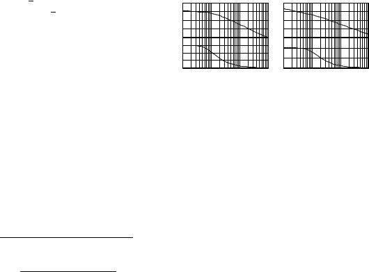
•For the plant without integrator whose static phase equals 0◦, selecting Φm = 90◦, under the condition (1), we obtain the phase plot of K(s)P (s) with a flat phase at −90◦ for all the frequencies below wc as shown in Fig. 1(a);
•For the plant with an integrator whose static phase equals −90◦, selecting Φm = 0◦, we obtain the phase plot of K(s)P (s) with a flat phase at −180◦ for all the frequencies below wc as shown in Fig. 1(b).
The above observations inform us that since we have already obtained a flat phase at −90◦ or −180◦, the only thing that needs to be done is just moving the flat phase to our desired phase requirement −π + Φm, which means we would better have a phase compensator with a constant phase Θ (−90◦ < Θ < 90◦) which is the most important characteristics of fractional order di erentiators or integrators sα (−1 < α < 1) (Manabe, 1961). Figure 2(a) gives the Bode plot of the fractional order integrator s−0.5 which has a constant phase at −45◦. Therefore, we can sim-
Bode Diagram
|
50 |
|
|
|
|
0 |
|
|
|
(dB) |
|
|
|
|
Magnitude |
−50 |
|
|
|
|
|
|
|
|
|
−100 |
|
|
|
|
−1500 |
|
|
|
|
−90 |
|
|
|
(deg) |
−180 |
|
|
|
Phase |
|
|
|
|
|
|
|
|
|
|
−270 |
|
|
|
|
−360 |
|
|
|
|
10−1 |
100 |
101 |
102 |
|
|
Frequency |
(rad/sec) |
|
Bode Diagram
|
50 |
|
|
|
|
0 |
|
|
|
(dB) |
|
|
|
|
Magnitude |
−50 |
|
|
|
|
|
|
|
|
|
−100 |
|
|
|
|
−135−150 |
|
|
|
Phase (deg) |
−180 |
|
|
|
−225 |
|
|
|
|
|
|
|
|
|
|
−270 |
|
|
|
|
10−1 |
100 |
101 |
102 |
|
|
Frequency |
(rad/sec) |
|
(a) The flat phase region of |
(b) The flat phase region of |
||||
1 |
|
1 |
|
||
K (s)P (s) (P (s) = |
|
) |
K (s)P (s) (P (s) = |
|
) |
(s+1)5 |
s(s+1)3 |
||||
for lower frequencies |
for lower frequencies |
||||
Fig. 1. Comparisons of the achieved flat phase regions for plants with and without an integrator
ply select the phase shaper as a fractional order di erentiator/integrator.
3.THE PHASE SHAPER
3.1FOC Approximation
From the discussions in the previous section, clearly, the phase shaper comes from the idea of FOC (Fractional Order Calculus) (Oustaloup
et al., 1996; Podlubny, 1999; Raynaud and Zerga¨ınoh, 2000; Vinagre and Chen, 2002). However, in practice, fractional order integrators or di erentiators can not exactly be achieved or implemented with the ideal Bode plot shown in Fig. (2)(a) because they are infinite dimensional linear filters. A bandlimit FOC implementation is important in practice, i.e., the finite-dimensional approximation of FOC should be done in a proper range of frequencies of practical interest (Chen and Moore, 2002; Oustaloup et al., 2000). Therefore, we can only design a phase compensator having a constant phase within a proper frequency range of interest.
In general, there are several approximation methods for FOC which can be divided into discretization method and frequency domain fitting method (Oustaloup et al., 2000; Chen et al., 2003b). Oustaloup proposed a continuous time frequency domain fitting method (Oustaloup et al., 2000) that can directly give the approximate s-transfer function. The existing discretization methods, e.g., (Machado, 1997; Vinagre et al., 2001), applied the direct power series expansion (PSE) of the Euler operator, continuous fractional expansion (CFE) of the Tustin operator and numerical integration based method.
3.2 Phase Shaper Realization
In designing a phase shaper, two factors in selecting the approximation method should be considered:
1)The phase shaper has a flat phase within the desired frequency range;
2)the phase shaper should have a lower order.
Therefore, in our study, a fourth order continued fraction expansion (CFE) of Tustin operator is employed which can give us a satisfying approximation result. The obtained discretized approximation of the fractional order integrator s−0.5 with the discretization sampling time Ts = 0.1s is give by
C(z) = 3.578z4 + 1.789z3 − 2.683z2 − 0.894z + 0.224 .(8) 16z4 − 8z3 − 12z2 + 4z + 1
which its Bode plot shown in Fig. 2(b).
100 |
|
|
|
|
|
50 |
|
|
|
|
|
0 |
|
|
|
|
|
−50 |
|
|
|
|
|
−100 |
|
|
|
|
|
10−2 |
10−1 |
100 |
101 |
102 |
103 |
0
−20
−40
−60
−80
−100
10−2 |
10−1 |
100 |
101 |
102 |
103 |
(a) The Bode plot of s−0.5 (continuous)
Bode Diagram
|
10 |
|
5 |
|
0 |
|
−5 |
(dB) |
−10 |
Magnitude |
−15 |
−20 |
|
|
|
|
−25 |
|
−30 |
|
−35 |
|
−400 |
(deg) |
−30 |
|
|
|
|
Phase |
|
|
|
|
|
|
|
|
|
|
|
|
−60 |
|
|
|
|
|
10−2 |
10−1 |
100 |
101 |
102 |
|
|
|
Frequency (rad/sec) |
|
|
(b) |
The |
Bode |
plot |
of |
|
s−0.5(discretized)
Fig. 2. Comparison of Bode plots for s−0.5 and the discretized approximation using CFE of Tustin operator (4/4)
From Fig. 2(b).it is seen that the phase of (8) is nearly constant at −45◦ within the frequency range between 4 rad./sec. and 30 rad./sec. The position of the constant phase area is greatly related with the discretization sampling time Ts and the width of that area shown on the Bode plot is fixed. To make the analysis more convenient, we transform the z-transfer function (8) to the s-transfer function (9) using the Tustin operator.
C(s) = 0.025s4 + 17.9s3 + 1252s2 + 1.67e004s + 3.58e004 (9) s4 + 186.7s3 + 5600s2 + 3.2e004s + 1.78e004
The Bode plot of (9) is shown in Fig. 3. The transfer function (9) shows us an illustrative example of a phase shaper with the property of locally constant phase Θ (−90◦ < Θ < 90◦). The position of the constant phase region is adjustable
Bode Diagram
|
10 |
|
0 |
(dB) |
−10 |
Magnitude |
−20 |
|
|
|
−30 |
|
−40 |
|
0 |
(deg) |
−30 |
|
Phase |
||
|
−60
10−1 |
100 |
101 |
102 |
103 |
104 |
|
|
|
Frequency (rad/sec) |
|
|
Fig. 3. Bode plot of the continuous-time fourth order approximation using CFE of the Tustin operator
by selecting di erent Ts. Combining the PID controller K(s) which makes the system K(s)P (s) have a flat phase in the lower frequency area, the phase shaper C(s) can be used to ensure that the open loop system C(s)K(s)P (s) has the flat phase with the expected width centered at the desired position. It is obvious that the constant phase area of C(s) and the flat phase area of K(s)P (s) must have an intersection and wc for the PID controller design turns into the upper limit of the flat phase of the open loop system and the lower limit of the
flat phase is determined roughly by 1 rad./sec.
10Ts
4. DESIGN PROCEDURE
As discussed in Sec. 2, the PID controller and the phase shaper are designed separately. In what follows, the design procedures will be summarized
4.1 PID Controller Design
How to determine sp(wc) was discussed in (Chen et al., 2003a) based on the experimental measurement of 6 P (jwc) and |P (jwc )|. Therefore, let us summarize what are known at this point for PID controller design. We are given i) wc; ii) Φm = 90◦ or 180◦; iii) measurement of 6 P (jwc ) and |P (jwc)| (Chen et al., 2003a) and iv) an estimation of sp(wc ) (Chen et al., 2003a).
Then, using (5), (6) and (7), we can retrieve the PID parameters Kp, Ti and Td.
4.2 Phase Shaper Design
The steps for designing phase shaper include i) selecting α, based on the phase margin requirement for the open loop system, for the fractional order integrator or di erentiator sα; ii) calculating the approximation transfer function for the fractional order integrator or di erentiator; iii) selecting a proper discretization sampling time Ts to determine the position of the constant phase area of the approximation transfer function.
4.3 Gain Adjustment
Note that, among the above design procedures, only the phase requirement for the open loop system C(s)K(s)P (s) is considered. However, we also need to care about the gain so that the sensitivity circle touches the flat phase region of the Nyquist curve exactly and the gain crossover frequency is settled within the flat phase. Therefore, a gain β is used to match the gain condition
G(jwgc ) = βC(jwgc )K(jwgc )P (jwgc ) = 1.(10)

where wgc is the desired gain crossover frequency
of the open loop system ( 1 < wgc < wc ). It is
10Ts
suggested to select wgc at the midpoint of the flat phase area.
Equivalently, we use βC(s) to update C(s) so that the open loop system C(s)K(s)P (s) matches both of the phase and gain requirement.
4.4 Selection of wc and Ts
Because wc and Ts determine the width and the position of the flat phase, it is very important to give a guidance to select wc and Ts. Two factors influence the selections of wc and Ts: 1) the desired gain crossover frequency wgc should be within the flat phase region; 2) the flat phase area may not be so wide as well, i.e., the width is below 0.2 rad./sec. For better performance, it is suggested that wc <0.3 rad./sec.
5. ILLUSTRATIVE SIMULATION
The modified tuning method presented above will be illustrated via some simulation examples. In the simulation, the following classes of plants, studied in (Wall´en et al., 2002), will be used.
Pn (s) = |
|
|
|
1 |
|
|
|
, n = 1, 2, 3, 4; |
(11) |
|||||
|
|
|
|
|
|
|
||||||||
|
|
|
|
|
(n+3) |
|||||||||
|
(s + 1) |
|
|
|
|
|
|
|
||||||
P5 |
(s) = |
|
|
1 |
|
|
; |
|
(12) |
|||||
|
|
|
|
|
|
|||||||||
s(s |
|
3 |
|
|||||||||||
|
|
|
|
|
|
|
+ 1) |
|
|
|
||||
P6 |
(s) = |
1 |
|
|
e−s; |
(13) |
||||||||
|
|
|
|
|
||||||||||
|
|
|
|
4 |
||||||||||
|
|
|
|
|
|
(s + 1) |
|
|
||||||
P7 |
(s) = |
|
1 |
|
|
|
e−s |
; |
(14) |
|||||
|
|
|
|
|
|
|||||||||
|
|
|
|
|
3 |
|||||||||
|
|
|
|
|
s(s + 1) |
|
|
|||||||
5.1 The General Plant P2(s)
We still consider P2(s) in (11) first, which was studied in (Wall´en et al., 2002; Chen et al., 2003a). For the PID controller design, because the plant P2(s) does not include any integrator, Φm should be set as 90◦ and wc = 0.25 rad./sec. With these specifications, the PID controller K2(s) is designed as
1
K2(s) = 1.095(1 + 4.892s + 1.829s). (15)
The specifications of the phase shaper C2(s) are set as α = −0.5, which means that we use the fractional order integrator s−0.5 as the original form of the phase shaper, Ts = 1 sec. and β =
Bode Diagram
|
100 |
|
|
|
|
|
|
|
50 |
|
|
|
|
|
|
|
0 |
|
|
|
|
|
|
(dB) |
−50 |
|
|
|
|
|
|
|
|
|
|
|
|
|
|
Magnitude |
−100 |
|
|
|
|
|
|
−150 |
|
|
|
|
|
|
|
|
−200 |
|
|
|
|
|
|
|
−250 |
|
|
|
|
|
|
|
−300−90 |
|
|
|
|
|
|
|
−180 |
|
|
|
|
|
|
(deg) |
−270 |
|
|
|
|
|
|
Phase |
|
|
|
|
|
|
|
|
|
|
|
|
|
|
|
|
−360 |
|
|
|
|
|
|
|
−450 |
|
|
|
|
|
|
|
10−3 |
10−2 |
10−1 |
100 |
101 |
102 |
103 |
|
|
|
|
Frequency (rad/sec) |
|
|
|
Fig. 4. Bode diagram comparison (Dashed line: The modified Ziegler-Nichols; Dotted line: “Flat phase” PID; Solid line: The proposed.)
Nyquist Diagram
|
1 |
|
|
|
|
|
|
|
|
|
0.5 |
|
|
|
|
|
|
|
|
|
0 |
|
|
|
|
|
|
|
|
|
−0.5 |
|
|
|
|
|
|
|
|
Axis |
|
|
|
|
|
|
|
|
|
Imaginary |
−1 |
|
|
|
|
|
|
|
|
|
−1.5 |
|
|
|
|
|
|
|
|
|
−2 |
|
|
|
|
|
|
|
|
|
−2.5 |
|
|
|
|
|
|
|
|
|
−3 |
|
|
|
|
|
|
|
|
|
−3 |
−2.5 |
−2 |
−1.5 |
−1 |
−0.5 |
0 |
0.5 |
1 |
Real Axis
Fig. 5. Nyquist diagram comparison (Dashed line: The modified Ziegler-Nichols; Dotted line: “Flat phase” PID; Solid line: The proposed.)
9.091. The phase shaper designed by the proposed method is
|
|
0.0226s4 |
+ 1.626s3 |
+ 11.38s2 + 15.18s + 3.252 |
||
C2 |
(s) = |
|
|
|
|
.(16) |
s4 + 18.67s3 |
+ 56s2 |
|
||||
|
|
+ 32s + 1.778 |
||||
For comparison, the corresponding PID controller designed by the modified Ziegler-Nichols method is K2z = 0.232(1 + + 0.253s) while the corresponding PID controller designed by the “flat phase” tuning method (Chen et al., 2003a) is
K2f = 0.671(1 + 1 + 1.657s).
2.149s
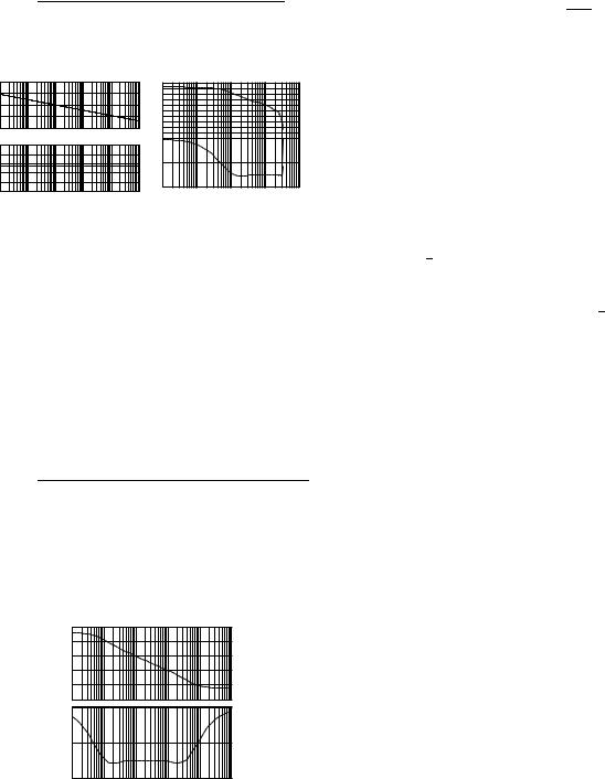
The Bode and the Nyquist plots are compared in Figs. 4 and 5.
From Fig. 4, it is seen that the phase plot between 0.1 rad./sec. and 0.3 rad./sec. is flat. The phase margin roughly equals 45◦. In Fig. 5, the Nyquist curve of the open loop system is tangential to the sensitivity circle at the flat phase. And we can also see that the flat phase is wide enough to accommodate the gain variation of the plant. The step responses of the closed-loop systems are compared in Fig. 6. Comparing the closed-loop system with the proposed modified controller to that with the modified Ziegler-Nichols controller, the overshoots of the step response from the proposed scheme remain invariant under gain variations. However, the overshoots of the modified Ziegler-Nichols controller change remarkably.
Step Response
1.5 |
|
|
|
|
|
|
|
|
|
1 |
|
|
|
|
|
|
|
|
|
Amplitude |
|
|
|
|
|
|
|
|
|
0.5 |
|
|
|
|
|
|
|
|
|
0 |
|
|
|
|
|
|
|
|
|
0 |
20 |
40 |
60 |
80 |
100 |
120 |
140 |
160 |
180 |
|
|
|
|
|
Time (sec) |
|
|
|
|
Step Response
1.4 |
|
|
|
|
|
|
|
|
|
1.2 |
|
|
|
|
|
|
|
|
|
1 |
|
|
|
|
|
|
|
|
|
0.8 |
|
|
|
|
|
|
|
|
|
Amplitude |
|
|
|
|
|
|
|
|
|
0.6 |
|
|
|
|
|
|
|
|
|
0.4 |
|
|
|
|
|
|
|
|
|
0.2 |
|
|
|
|
|
|
|
|
|
0 |
|
|
|
|
|
|
|
|
|
0 |
20 |
40 |
60 |
80 |
100 |
120 |
140 |
160 |
180 |
|
|
|
|
|
Time (sec) |
|
|
|
|
(a) Step responses of the (b) Step response of the closed-loop system with the closed-loop system with the modified Ziegler-Nichols “flat phase” PID controller and the “flat phase” PID plus a phase shaper controllers
Fig. 6. Comparisons of step responses (Dashed line: The modified Ziegler-Nichols; Dotted line: “Flat Phase” PID; Solid line: The proposed. For all schemes, gain variations 1, 1.1,
1.3are considered in step responses)
5.2Plant With An Integrator P5(s)
This case is omitted due to space limitation. Please refer to the combined case in Sec. 5.4.
5.3 Plant With A Time Delay P6(s)
This case is omitted due to space limitation. Please refer to the combined case in Sec. 5.4.
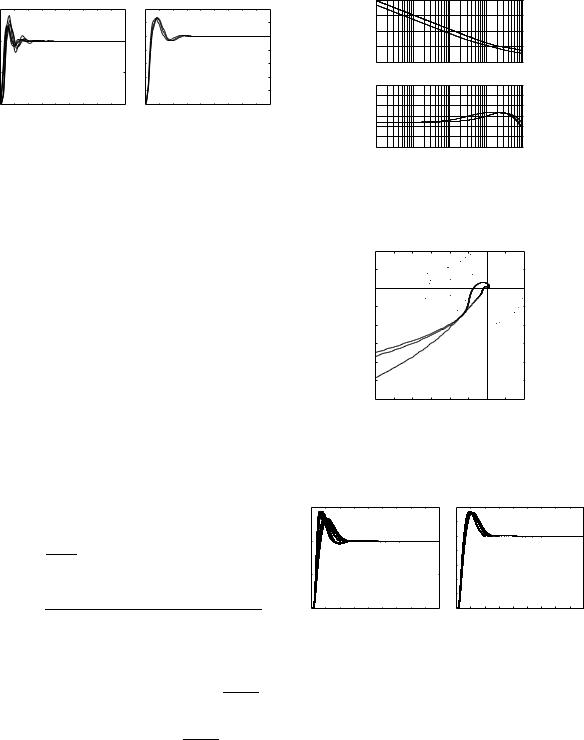
5.4 Plant With An Integrator And A Time Delay
P7(s)
For the plant with an integrator and a time delay P7(s), the proposed PID controller is K7(s) =
0.228(1 + 1 + 1.343s) with respect to wc=0.25
4.002s
rad./sec. and Φm=0◦. The proposed phase shaper is
4.528s4 + 56.35s3 + 112.7s2 + 42.93s + 1.59 C7(s) = 0.5062s4 + 24.3s3 + 113.4s2 + 100.8s + 14.4
with respect to α = 0.5, Ts = 1.5 sec. and β = 0.022.
The controller designed by the modified Ziegler-
Nichols method is K7z = 0.266(1 + 1 +
10.136s
2.534s). The corresponding PID controller designed by the “flat phase” tuning method (Chen
et al., 2003a) is K7f = 0.268(1 + 1 + 2.438).
10.795s
6. CONCLUSION
This paper presents an extension of our previous work where a robust PID autotuning method was proposed by using the idea of “flat phase”, i.e., the phase derivative w.r.t. the frequency is zero at a given frequency called the “tangent frequency” so that the closed-loop system is robust to gain variations and the step responses exhibit an isodamping property. However, the width of the achieved phase flatness region is hard to adjust.
300 |
|
|
|
200 |
|
|
|
100 |
|
|
|
0 |
|
|
|
−100 |
10−2 |
10−1 |
100 |
10−3 |
|||
0 |
|
|
|
−50 |
|
|
|
−100 |
|
|
|
−150 |
|
|
|
−200 |
|
|
|
−250 |
|
|
|
−300 |
10−2 |
10−1 |
100 |
10−3 |
Fig. 7. System With Integrator And Delay: Bode diagram comparison (Dashed line: The modified Ziegler-Nichols; Dotted line: “Flat Phase” PID; Solid line: The proposed)
1 |
|
|
|
|
|
|
|
|
0.5 |
|
|
|
|
|
|
|
|
0 |
|
|
|
|
|
|
|
|
−0.5 |
|
|
|
|
|
|
|
|
−1 |
|
|
|
|
|
|
|
|
−1.5 |
|
|
|
|
|
|
|
|
−2 |
|
|
|
|
|
|
|
|
−2.5 |
|
|
|
|
|
|
|
|
−3 |
−2.5 |
−2 |
−1.5 |
−1 |
−0.5 |
0 |
0.5 |
1 |
−3 |
Fig. 8. System With Integrator And Delay: Nyquist diagram comparison (Dashed line: The modified Ziegler-Nichols; Dotted line: “Flat Phase” PID; Solid line: The proposed)
1.5 |
|
|
|
|
|
|
|
|
|
1.4 |
|
|
|
|
|
|
|
|
|
|
|
|
|
|
|
|
|
|
|
1.2 |
|
|
|
|
|
|
|
|
|
|
|
|
|
|
|
|
|
|
|
1 |
|
|
|
|
|
|
|
|
|
1 |
|
|
|
|
|
|
|
|
|
|
|
|
|
|
|
|
|
|
|
|
|
|
|
|
|
|
|
|
|
0.8 |
|
|
|
|
|
|
|
|
|
|
|
|
|
|
|
|
|
|
|
0.6 |
|
|
|
|
|
|
|
|
|
0.5 |
|
|
|
|
|
|
|
|
|
|
|
|
|
|
|
|
|
|
|
|
|
|
|
|
|
|
|
|
|
0.4 |
|
|
|
|
|
|
|
|
|
|
|
|
|
|
|
|
|
|
|
0.2 |
|
|
|
|
|
|
|
|
|
0 |
20 |
40 |
60 |
80 |
100 |
120 |
140 |
160 |
180 |
0 |
20 |
40 |
60 |
80 |
100 |
120 |
140 |
160 |
180 |
0 |
0 |
(a) Step Responses of sys- (b) Step response of system tem with Modified Zieglerwith phase shaper
Nichols controller and “flat phase” PID controller
Fig. 9. System With An Integrator And A Time Delay: Comparisons of step responses (Dashed line: The modified Ziegler-Nichols; Dotted line: “Flat Phase” PID; Solid line: The proposed. For all schemes, gain variations 1, 1.1, 1.3 are considered in step responses)
A phase shaping idea is proposed to make the width of the phase flatness region adjustable. With a suitable phase shaper, we are able to determine the width of the flat phase region so as to make the whole design procedure of a robust PID controller much easier and the system performance can be enhanced more significantly. The plant gain and phase at the desired frequency, which are identified by several relay feedback tests

in an iterative way, are used to estimate the derivatives of the amplitude and phase of the plant with respect to the frequency at the same frequency point by the well known Bode’s integral relationship. Then, these derivatives are used to design the proposed robust PID controller. The phase shaper, based on the idea of FOC (Fractional Order Calculus), is actually a fractional order integrator or di erentiator. In this paper, no plant model is assumed during the controller design. Only several relay tests and calculations are needed. Simulation examples illustrate the e ectiveness and the simplicity of the proposed method with an iso-damping property. From the illustrative simulation, it can be seen that the proposed phase shaping approach to robust PID controller tuning gives a satisfying performance for a class of plants.
Our further research e orts include 1) Testing on more types of plants; 2) Experiment on real plants 3) Exploration of nonminimum phase, open loop unstable systems.
7. ACKNOWLEDGMENTS
The authors are grateful to Professor Li-Chen Fu, Editor- in-Chief of Asian Journal of Control for providing a complimentary copy of the “Special Issue on Advances in PID Control”, Asian J. of Control (vol. 4, no. 4). The simulation study was helped by C. H. Hu.
REFERENCES
Karl J. Astrom and Tore Hagglund. PID Controllers: Theory, Design, and Tuning. ISA - The Instrumentation, Systems, and Automation Society (2nd edition), 1995.
Y. Q. Chen, C. H. Hu, and K. L. Moore. Relay feedback tuning of robust PID controllers with iso-damping property. In Proceedings of The 42nd IEEE Conference on Decision and Control, Hawaii, 2003a.
Y. Q. Chen and K. L. Moore. Discretization schemes for fractional-order di erentiators and integrators. IEEE Trans. Circuits Syst. I, 49:363–367, March 2002.
YangQuan Chen, B. M. Vinagre, and Igor Podlubny. On fractional order disturbance observers. In Proc. of
The First Symposium on Fractional Derivatives and Their Applications at The 19th Biennial Conference on Mechanical Vibration and Noise, the ASME International Design Engineering Technical Conferences & Computers and Information in Engineering Conference (ASME DETC2003), pages 1–8, DETC2003/VIB--48371, Chicago, Illinois, 2003b.
C. C. Hang, K. J. ˚Astr¨om, and W. K. Ho. Refinements of the Ziegler-Nichols tuning formula. IEE Proc. Pt. D, 138(2):111–118, 1991.
A.Karimi, D. Garcia, and R. Longchamp. Iterative controller tuning using Bode’s integrals. In Proceedings of the 41st IEEE Conference on Decision and Control, pages 4227–4232, Las Vegas, Nevada, 2002a.
A.Karimi, D. Garcia, and R. Longchamp. PID controller design using Bode’s integrals. In Proceedings of the American Control Conference, pages 5007–5012, Anchorage, AK, 2002b.
B. Kristiansson and B. Lennartsson. Optimal PID controllers including roll o and Schmidt predictor structure. In Proceedings of IFAC 14th World Congress, volume F, pages 297–302, Beijing, P. R. China, 1999.
J. A. T. Machado. Analysis and design of fractionalorder digital control systems. J. Syst. Anal. ModelingSimulation, 27:107–122, 1997.
S.Manabe. The non-integer integral and its application to control systems. ETJ of Japan, 6(3-4):83–87, 1961.
A.Oustaloup, F. Levron, F. Nanot, and B. Mathieu. Frequency band complex non integer di erentiator: Characterization and synthesis. IEEE Trans. Circuits Syst. I, 47:25–40, Jan. 2000.
A.Oustaloup, X. Moreau, and M. Nouillant. The crone
suspension. Control Eng. Pract., 4(8):1101–1108, 1996. H. Panagopoulos, K. J. ˚Astr¨om, and T. H¨agglund. Design of PID controllers based on constrained optimization. In
Proceedings of the American Control Conference, San Diego, CA, 1999.
Igor Podlubny. Fractional-order systems and PIλ Dµ- controllers. IEEE Trans. Automatic Control, 44(1):208– 214, 1999.
H. F. Raynaud and A. Zerga¨ınoh. State-space representation for fractional order controllers. Automatica, 36(7): 1017–1021, 2000.
K. K. Tan, T. H. Lee, and Q. G. Wang. Enhanced automatic tuning procedure for process control of PI/PID controllers. AlChE Journal, 42(9):2555–2562, 1996.
B.M. Vinagre, I. Petras, P. Merchant, and L. Dorcak. Two digital realization of fractional controllers: Application
to temperature control of a solid. In in Proc. Eur. Control Conf. (ECC01), pages 1764–1767, Porto, Portugal, 2001.
Blas M. Vinagre and YangQuan Chen. Lecture note on fractional calculus applications in automatic control and robotics. In Blas M. Vinagre and YangQuan Chen, editors, The 41st IEEE CDC2002 Tutorial Workshop # 2, pages 1– 310. [Online] http://mechatronics.ece.usu.edu /foc/cdc02 tw2 ln.pdf, Las Vegas, Nevada, USA, 2002.
A. Wall´en, K. J. ˚Astr¨om, and T. H¨agglund. Loop-shaping design of PID controllers with constant ti /td ratio.
Asian Journal of Control, 4(4):403–409, 2002.