Design of an active acoustic sensor system for an autonomous underwater vehicle

Chapter 6 Hardware Verification and Experimental Results

Detection Range for the Echo

Sounder

precentage detection (%)

120

100

80

60

40

20

0

0

1

2

3

4

5

distance to the surface (m)

Figure 6.12: Detection of an echo for different distances

There are a number of factors that affect the attenuation of the signal in the water. These have been discussed thoroughly in Chapter 2. The key factors that result in highly attenuated signals at the receiver are:

•The low intensity of the transmitted signal

•The signal’s susceptibility, at 200 kHz, to losses due to bulk viscosity and absorption due to relaxation

•The wall’s reflectivity, which will result in only some of the signal being reflected by the wall whilst the rest is transmitted through the wall

•The natural attenuation of the signal in the medium due to absorption and scattering

This clearly is not the distance that the transducer is capable of achieving and does not meet the requirement of 5m, as stated in chapter 3. The Navman echo sounder circuit that the transducer was taken from can achieve a distance of up to 184m. The LM1812 ultrasonic transceiver chip is capable of depth sounding up to 30m. This clearly indicates that not enough power is being converted to acoustic energy at the transmitter stage.

6.2.6 Investigation of Signal Transmission Intensity

There were three possible reasons for the lack of signal transmission intensity. These were:

•The key input voltage to the LM1812 chip in not high enough

•The LC resonator has not been correctly tuned to 200 kHz

57

Design of an Active Acoustic Sensor System

•There is a problem with stepping the voltage up to the required level for the transducer.

One concern was that the 5V pulse from the Eyebot did not have enough voltage to meet the 12V suggested in the LM1812 datasheet [14]. A simple test was conducted to determine if this may have resulted in a weaker signal transmitted by the echo sounder. The following circuit is connected between the digital output of the Eyebot and the echo sounder.

Figure 6.13: Driver circuit to increase the voltage at the input of echo sounder

Figure 6.14 is the display of the oscilloscope when no driver is used. Figure 6.15 is the display when a driver is used. The signals have been inverted so that they can be easily captured by the oscilloscope. If the amplitude was increased, the transducer should ring much longer, resulting in the logic output being low for longer. As can be seen in the figures, the increase in voltage has not resulted in a wider logic output pulse. This means the key input voltage can be discounted as a factor for the lack of signal intensity.

Figure 6.14: Oscilloscope display for when no driver is used

58

Chapter 6 Hardware Verification and Experimental Results

Figure 6.15: Oscilloscope display for when driver is used

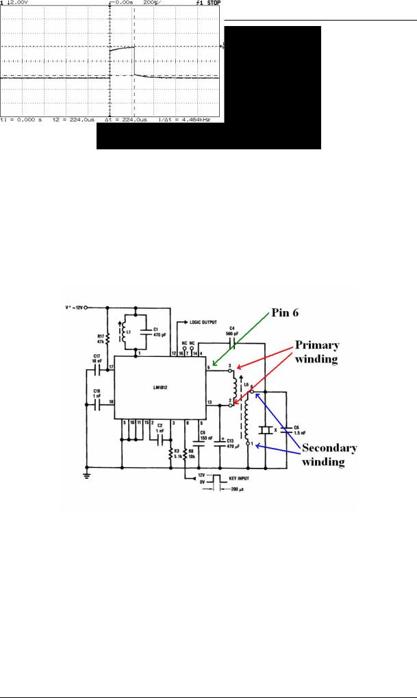
Another possible problem could have been that the LC resonator was not correctly tuned. Since the resonant frequency of the transducer is 200 kHz, this frequency must be exactly attained by the LC resonator. To conduct a test for this, the oscilloscope was connected to pin 6 of the LM1812 chip, which is shown in Figure 6.16. Pin 6 is the output signal to the transducer, from the chip. A pulse was then keyed from the Eyebot.

Figure 6.16: Location of pin 6 and transformer windings on the circuit diagram [14]

Figure 6.17 shows the result of the experiment. The measured frequency of the output from the LM1812 chip is exactly 200 kHz, which indicates that the LC resonator has been tuned correctly.

59

Design of an Active Acoustic Sensor System

Figure 6.17: Frequency of LM1812 output

The final possible cause for the lack of signal intensity is that the voltage signal to the transformer, which drives the transducer, is not stepped up to the right amplitude. If there is a problem at the step-up transformer stage, then there will not be significant lack of signal intensity for transmission. The test was conducted using the following procedure.

•Connect the oscilloscope across the primary windings of the transformer, shown in Figure 6.16, and key a pulse from the Eyebot to determine the peak-peak voltage (Vp-

p)of the input to the transformer. Repeat this, connecting the oscilloscope across the secondary windings of the transformer to determine the Vp-p of the output of the transformer.

Figure 6.18: Peak-peak voltage of transformer input

Figure 6.19: Peak-peak voltage of transformer output

60

Chapter 6 Hardware Verification and Experimental Results

Figures 6.18 and 6.19 show the observations of this experiment. As can be seen from the figures, there voltage has only been stepped up from 20.63Vp-p to 30.78Vp-p. However, the transformer has been designed with a turns ratio of 4.5:1. This means that the voltage should be stepped up by a factor of 4.5. This clearly is not the case.

The problem may be that the transformer does not properly match the source impedance to the load impedance of the transducer at 200 kHz. When these are matched, then there is maximum power transfer to the transducer. If the load and source impedance are given as:

RL = V2

I2

RS = V1

I1

And the transformer equations are:

V1 = N1 V2

N2

I1 = N2 I2

N1

(6.8)

(6.9)

where N1 and N2 are primary and secondary windings respectively, then the impedances can be matched by adjusting the windings to suit the following equation:

	N1		2	(6.10)
			RL
RS =	N2

To solve this impedance mismatch problem, the transformer’s windings need to be adjusted so that equation 6.10 is correctly met.

There are two other solutions possible that target the intensity of the signal, one implemented at the transmitter and one implemented at the receiver. The first is to develop a pulse amplifier that will increase the intensity of the signal at the transmitter. The second solution is to have a larger gain at the receiver to detect the smaller intensity signals. This can be achieved through a time variable attenuator. Both of these will be discussed in Chapter 8.

6.2.7 Time Redundancies for a Simple Fault Tolerant System

For the data seen in Table 6.1, it is clear that a fault tolerant system needs to be implemented to ensure that there is minimal probability of erroneous readings from the sensor.

61

Design of an Active Acoustic Sensor System

A simple system is implemented for the echo sounder based on the mid-value select method for choosing data points. The mid-value select method selects the median value from three readings to attempt to eliminate the chance of returning an outlying data point. In this case, the three values will be consecutive readings from the echo sounder. This will utilise the time redundancies to improve the estimate for distance.

The problem with a mid value select method is that the data returned by the echo sounder will have outliers lower than the true value. A much better approach is to choose the maximum from a set of three data points. This, too, is flawed in that it still may be possible to achieve an outlier above the true value.

A new method for fault tolerance is proposed. This involves the use of a pre-filter to remove most of the lower outliers. The pre-filter is just the maximum value from a number, selected by the user, of consecutive readings from the echo sounder. This is performed three times to obtain three maximum values. The median value of these three values is then selected to ensure that any higher outliers are not selected.

Distance														Detection
(m)						Samples								Percentage
2		10232		10242		10241		10231			10228			100
		10243		10240		10245		10245			10228
2.2		11447		11449		11448		11449			11465			100
		11449		11449		11449		11450			11449
2.4		12744		12747		12801		12745			12746			100
		12745		12799		12746		12746			12746
2.6		13807		13828		13824		13810			13822			100
		13809		13810		13822		13808			13809
2.8		14968		14967		14967		14968			14968			100
		14966		14968		14968		14968			14966
3		16104		16106		16116		16103			16103			100
		16102		16103		16102		16102			16102
3.2		17251		17254		17250		17251			17253			100
		17256		17250		17249		17250			17251
3.4		18352		18353		18356		18352			18350			100
		18352		18352		18354		18351			18349
3.6		19457		19424		19424		19423			19423			100
		19423		19422		19437		19412			19423
3.8		20579		20571		20581		20578			20580			100
		20580		20578		20579		20576			20575
4		21606		21610		21608		21586			21620			60
		1724		1724		21607		1699			1991
4.2		22791		22763		11442		22742			22756			90
		22767		6906		22742		11668			22743
4.4		1661		1672		1671		1689			1676			0
		1656		1724		1664		1676			1674

Table 6.2: Samples of sonar returns using extended mid-value select method

62

Chapter 6 Hardware Verification and Experimental Results

Table 6.2 shows the percentage detection over the range of distances measured for Table 6.1 using a pre-filter of size 3. This means that a maximum is chosen from three consecutive readings. It can be seen that, whilst the fault tolerance implemented does not increase the detectable range by much, it allows a virtually flawless detection rate over the entire detectable range.

This method of fault tolerance may take approximately nine times longer to process than just obtaining one reading, but it allows sonar returns to be more continuous, which is essential for navigational purposes. The pre-filter can be shortened if less time for processing is necessary. The form of fault tolerance implementation only has significant merit in the static cases, as is discussed in the next section.

6.3 Performance of the Sensor in a Dynamic Environment

The final part of this chapter deals with the performance of the echo sounder at tracking objects that move, or when the echo sounder is moving. Up until now, the tests performed on the echo sounder involved static experiments where the echo sounder was placed a certain distance from a wall and the time of flight measured.

This final experiment deals with a fixed transducer position in the water, with the transducer pointed into free space. A moving wooden rod is placed in from of the transducer and is moved back and forth in front of the transducer. The distance measurement is recorded and stored in an array, ready for uploading to a PC upon completion of the measurement stage. The points are then plotted on to a graph.

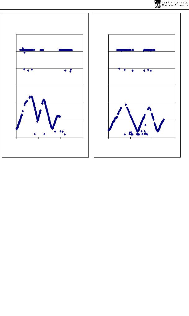
A new code set has been written for this experiment with the timing out of the channels, as is seen in the flow chart in Chapter 5, accounted for in assembly and C functions. Figures 6.20 and 6.21 show the graphs of the experiment. The data set is collected using the modified midvalue select method.

63

Design of an Active Acoustic Sensor System

Tracking the Stick 1

	6
	5
	4
(m)
distance	3
	2
	1
	0
	0	50	100	150	200	250

time (samples)

Figure 6.20: Distance wooden rod is from sensor over time

Tracking the Stick 2

	6				6
	5				5
	4				4
(m)				(m)
distance	3			distance	3
	2				2
	1				1
	0				0
	0	200	400	600

time (samples)

Tracking the Stick 3

0

200

400

600

time (samples)

Figure 6.21 a) & b): Measuring distance from the rod over 500 time samples

64

Chapter 6 Hardware Verification and Experimental Results

What can be seen from these graphs is that even with the implementation of a simple fault tolerant system, it is not possible to achieve zero errors in measurement.

The reason for this is that the obstacle is moving creating turbulence in the water. This turbulence will distort the echo’s frequency by adding random noise to the signal. As the circuit is tuned to 200 kHz, it will not be able to detect a significant distortion in frequency. Thus for the AUV to detect a wall or obstacle, it must be travelling at low speeds. This is ensured on the current AUV as the thrusters only allow low velocities. At the speeds the AUV will be travelling at, there should be minimal turbulence in the water. However, care must be taken to ensure that the sensors are not placed near areas of significant turbulence on the AUV, such as near the thrusters.

There is also another reason for the erroneous readings. The echo signal is subject to a phenomenon called the Doppler Effect. The Doppler Effect is when the observed frequency of the signal changes from the source frequency because the object is moving away or towards the source. The frequency of the observed signal becomes:

	∆f	=	vsource	(6.11)
	f		vsound

Since the Doppler Effect occurs both towards the rod and back to the sensor the formula can be written as:

	∆f	=	2vrod	(6.12)
	f		vsound

However, since the speed of the AUV will be very small with respect to the speed of sound, this effect is minimal in comparison to the effect that the turbulence has on the amount of erroneous readings.

At slow speeds, like in Figure 6.20, the sensor can track the rod well, with errors only when the rod is closer than the minimum detectable distance. This is compared with Figure 6.21 where the rod was moved much quicker. More errors are introduced as the sensor cannot detect the frequency properly.

An attempt is made to reduce the number of higher outliers by adjusting the modified midvalue select method. For this experiment, 10 samples are taken and the 7th sample in ascending order is taken as the estimated value. A) and b) of Figure 6.22 demonstrate the results of such an experiment.

65

Design of an Active Acoustic Sensor System

Tracking the Stick DMVS 1

	6				6
	5				5
	4				4
(m )				(m )
distance	3			distance	3
	2				2
	1				1
	0				0
	0	200	400	600

time (samples)

Tracking the Stick DMVS 2

0

200

400

600

time (samples)

Figure 6.22: 7th value select method on the tracking of a wooden rod

As can be seen from the plots, outliers from above the true value are removed, but are then replaced by outliers from below the true value. What this means is that it is impossible to remove all the outliers from being detected using this method of fault tolerance. However, using the earlier modified fault tolerance method, the percentage error is 20%, as opposed to 40%, for the latter, to 20%.

The errors may be reduced partially by investigating the population of data points to determine where the data, which is within 10% of the true value, lies in relation to the ordered data set. For example, if the investigation found that this data lies in the 80th percentile, then 10 sample points can be taken and sorted in ascending order, and the 8th data point will be the estimate of the data. This is an area for future investigation.

Obviously, the more data points collected, the better the robustness of the system, but this will result in a slower data rate. 10 sample points will result in a data rate of approximately 10Hz, which is the minimum requirement for this project, and thus should not be exceeded.

66