

Fang F.Lightweight floating-point arithmetic.Case study of IDCT
.pdfLightweight Floating-Point Arithmetic:
Case Study of Inverse Discrete Cosine Transform
Fang Fang, Tsuhan Chen, and Rob A. Rutenbar
Dept. of Electrical and Computer Engineering, Carnegie Mellon University
5000 Forbes Avenue, Pittsburgh, PA 15213, USA
Abstract - To enable floating-point (FP) signal processing applications in low-power mobile devices, we propose lightweight floating-point arithmetic. It offers a wider range of precision/power/speed/area tradeoffs, but is wrapped in forms that hide the complexity of the underlying implementations from both multimedia software designers and hardware designers. Libraries implemented in C++ and Verilog provide flexible and robust floating-point units with variable bit-width formats, multiple rounding modes and other features. This solution bridges the design gap between software and hardware, and accelerates the design cycle from algorithm to chip by avoiding the translation to fixed-point arithmetic. We demonstrate the effectiveness of the proposed scheme using the inverse discrete cosine transform (IDCT), in the context of video coding, as an example. Further, we implement lightweight floating-point IDCT into hardware and demonstrate the power and area reduction.
Keywords – floating-point arithmetic, customizable bitwidth, rounding modes, low-power, inverse discrete cosine transform, video coding
1. Introduction
Multimedia processing has been finding more and more applications in mobile devices. A lot of effort must be spent to manage the complexity, power consumption and time-to-market of the modern multimedia system-on-chip (SoC) designs. However, multimedia algorithms are computationally intensive, rich in costly FP arithmetic operations rather than simple logic. FP arithmetic hardware offers a wide dynamic range and high computation precision, yet occupies large fractions of total chip area and energy budget. Therefore, its application on mobile computing chip is highly limited. Many embedded microprocessors such as the StrongARM [1] do not include a FP unit due to its unacceptable hardware cost.
So there is an obvious gap in multimedia system development: software designers prototype these algorithms using high-precision FP operations, to understand how the algorithm behaves, while the silicon designers ultimately implement these algorithms into integer-like hardware, i.e., fixed-point units. This seemingly minor technical choice actually creates severe consequences: the need to use fixed-point operations often distorts the natural form of the algorithm, forces awkward design trade-offs, and even introduces perceptible artifacts. Error analysis and word-length optimization of fixedpoint 2D IDCT algorithm has been studied in [2], and a tool for translating FP algorithms to fixed-point algorithms was presented in [3]. However, such optimization and translation are based on
human knowledge of the dynamic range, precision requirements and the relationship between algorithm’s architecture and precision. This time-consuming and error-prone procedure often becomes the bottleneck of the entire system design flow.
In this paper, we propose an effective solution: lightweight FP arithmetic. This is essentially a family of customizable FP data formats that offer a wider range of precision/power/speed/area tradeoffs, but wrapped in forms that hide the complexity of the underlying implementations from both multimedia algorithm designers and silicon designers. Libraries implemented in C++ and Verilog provide flexible and robust FP units with variable bit-width formats, multiple rounding modes and other features. This solution bridges the design gap between software and hardware and accelerate the design cycle from algorithm to chip. Algorithm designers can translate FP arithmetic computations transparently to lightweight FP arithmetic and adjust the precision easily to what is needed. Silicon designers can use the standard ASIC or FPGA design flow to implement these algorithms using the arithmetic cores we provide which consume less power than standard FP units. Manual translation from FP algorithms to algorithms can be eliminated from the design cycle.
We test the effectiveness of our lightweight arithmetic library using a H.263 video decoder. Typical multimedia applications working with modest-resolution human sensory data such as audio and video do not need the whole dynamic range and precision that IEEE-standard FP offers. By reducing the complexity of FP arithmetic in many dimensions, such as narrowing the bit-width, simplifying the rounding methods and the exception handling, and even increasing the radix, we explore the impact of such lightweight arithmetic on both the algorithm performance and the hardware cost.
Our experiments show that for the H.263 video decoder, FP representation with less than half of the IEEE-standard FP bitwidth can produce almost the same perceptual video quality. Specifically, only 5 exponent bits and 8 mantissa bits for a radix- 2 FP representation, or 3 exponent bits and 11 mantissa bits for a radix-16 FP representation are all we need to maintain the video quality. We also demonstrate that a simple rounding mode is sufficient for video decoding and offers enormous reduction in hardware cost. In addition, we implement a core algorithm in the video codec, IDCT, into hardware using the lightweight arithmetic unit. Compared to a conventional 32-bit FP IDCT, our approach reduces the power consumption by 89.5%.
The paper is organized as follows: Section 2 introduces briefly the relevant background on FP and fixed-point representations. Section 3 describes our C++ and Verilog
libraries of lightweight FP arithmetic and the usage of the libraries. Section 4 explores the complexity reduction we can achieve for IDCT built with our customizable library. Based on the results in this section, we present the implementation of lightweight FP arithmetic units and analyze the hardware cost reduction in Section 5. In Section 6, we compare the area/speed/power of a standard FP IDCT, a lightweight FP IDCT and a fixed-point IDCT. Concluding remarks follow in Section 7.
2. Background
2.1 Floating-point representation vs. fixed-point representation
There are two common ways to specify real numbers: FP and fixed-point representations. FP can represent numbers on an exponential scale and is reputed for a wide dynamic range. The date format consists of three fields: sign, exponent and fraction (also called ‘mantissa’), as shown in Fig. 1:
1 |
8 |
23 |
s |
exp |
frac |
|
|
|
FP value: (-1)s 2 exp-bias * 1. frac ( The leading 1 is implicit) 0 ≤ exp ≤ 255, bias = 127
Fig.1. FP number representation
Dynamic range is determined by the exponent bit-width, and resolution is determined by the fraction bit-width. The widely
adopted IEEE single FP standard [4] uses a 8-bit exponent that can reach a dynamic range roughly from 2-126 to 2127 , and a 23-
bit fraction that can provide a resolution of 2exp-127 * 2-23, where ‘exp’ stands for value represented by the exponent field.
In contrast, the fixed-point representation is on a uniform scale that is essentially the same as the integer representation, except for the fixed radix point. For instance (see Fig. 2), a 32bit fixed-point number with a 16-bit integer part and a 16-bit
fraction part can provide a dynamic range of 2-16 to 216 and a resolution of 2-16.
16 |
16 |
int |
frac |
|
|
Fig.2. Fixed-point number representation
When prototyping algorithms with FP, programmers do not have to concern about dynamic range and precision, because IEEE-standard FP provides more than necessary for most general applications. Hence, ‘float’ and ‘double’ are standard parts of programming languages like C++, and are supported by most compilers. However, in terms of hardware, the arithmetic operations of FP need to deal with three parts (sign, exponent, fraction) individually, which adds substantially to the complexity of the hardware, especially in the aspect of power consumption, while fixed-point operations are almost as simple as integer operations. If the system has a stringent power budget, then the application of FP units has to be limited, and on the other hand, a lot of manual work is spent in implementing and optimizing the
fixed-point algorithms to provide the necessary dynamic range and precision.
2.2 IEEE-754 floating-point standard
IEEE-754 is a standard for binary FP arithmetic [4]. Since our later discussion about the lightweight FP is based on this standard, we give a brief review of its main features in this section.
Data format
The standard defines two primary formats, single-precision (32 bits) and double precision (64 bits). The bit-widths of three fields and the dynamic range of single and double-precision FP are listed in Table 1.
Format |
Sign |
Exp |
Frac |
Bias |
Max |
Min |
|
|
|
|
|
|
|
|
|
Single |
1 |
8 |
23 |
127 |
3.4 |
* 1038 |
1.4*10-45 |
|
|
|
|
|
|
|
|
Double |
1 |
11 |
52 |
1023 |
1.8 |
* 10308 |
4.9 *10-324 |
|
|
|
|
|
|
|
|
Table 1. IEEE FP number format and dynamic range
Rounding
The default rounding mode is round-to-nearest. If there is a tie for the two nearest neighbors, then it’s rounded to the one with the least significant bit as zero. Three user selectable rounding modes are: round-toward +∞, round-toward -∞, and round-toward-zero (or called truncation).
Denormalization
Denormalization is a way to allow gradual underflow. For normalized numbers, because there is an implicit leading ‘1’, the smallest positive value is 2-126 * 1.0 for single precision (it is not 2-127 * 1.0 because the exponent with all zeros is reserved for denormalized numbers). Values below this can be represented by a so-called denormlized format (Fig. 3) that does not have the implicit leading’1’.
1 |
8 |
23 |
s |
00000000 |
frac ≠0 |
|
|
|
Fig. 3. Denormalized number format
The value of the denormalized number is 2-126 * 0.frac and the smallest representable value is hence scaled down to 2-149 (2- 126 * 2-23). Denormalization provides graceful degradation of precision for computations on very small numbers. However, it complicates hardware significantly and slows down the more common normalized cases.
Exception handling
There are five types of exceptions defined in the standard: invalid operation, division by zero, overflow, underflow, and inexact. As shown in Fig. 4, some bit patterns are reserved for these exceptions. When numbers simply cannot be represented, the format returns a pattern called a “Nan” – Not-a-Number – with information about the problem. NaNs provide an escape

|
1 |
8 |
23 |
|
Infinite |
s |
11111111 |
frac == 0 |
|
|
|
|
|
|
NaN |
1 |
8 |
23 |
|
s |
11111111 |
frac ≠0 |
||
(Not-a-Number) |
||||
|
|
|
|
NaN is assigned when some invalid operations occur, like (+∞) + (-∞), 0 * ∞, 0 / 0 …etc
Fig. 4. Infinite and NaN representations
mechanism to prevent system crashes in case of invalid operations. In addition to assigning specific NaN bit patterns, some status flags and trapping signals are used to indicate exceptions.
From the above review, we can see that IEEE-standard FP arithmetic has a strong capability to represent real numbers as accurately as possible and is very robust when exceptions occur. However, if the FP arithmetic unit is dedicated to a particular application, the IEEE-mandated 32 or 64-bit long bit-width may provide more precision and dynamic range than needed, and many other features may be unnecessary as well.
3. Customizable Lightweight Floating-Point Library
The goal of our customizable lightweight FP library is to provide more flexibility than IEEE-standard FP in bit-width, rounding and exception handling. We created matched C++ and Verilog FP arithmetic libraries that can be used during algorithm/circuit simulation and circuit synthesis. With the C++ library, software designers can simulate the algorithms with lightweight arithmetic and decide the minimal bit-width, rounding mode, etc. according to the numerical performance. Then with the Verilog library, hardware designers can plug in the parameterized FP arithmetic cores into the system and synthesize it to the gate-level circuit. Our libraries provide a way to move the FP design choices (bit-width, rounding…) upwards to the algorithm design stage and better predict the performance during early algorithm simulation.
3.1 Easy-to-use C++ class ‘Cmufloat’ for algorithm designers
Our lightweight FP class is called ‘Cmufloat’ and implemented by overloading existing C++ arithmetic operators ( +, - , *, /…). It allows direct operations, including assignment between ‘Cmufloat’ and any C++ data types except char. The bitwidth of ‘Cmufloat’ varies from 1 to 32 including sign, fraction and exponent bits and is specified during the variable declaration. Three rounding modes are supported: round-to-nearest, Jamming, and truncation, one of which is chosen by defining a symbol in an appropriate configuration file. Explanation of our rounding modes is presented in detail later. In Fig. 5, we summarize the operators of ‘Cmufloat’ and give some examples of using ‘Cmufloat’.
Our implementation of lightweight FP offers two advantages. First, it provides a transparent mechanism to embed ‘Cmufloat’ numbers in programs. As shown in the example, designers can use ‘Cmufloat’ as a standard C++ data type. Therefore, the overall structure of the source code can be preserved and a
minimal amount of work is spent in translating a standard FP program to a lightweight FP program. Second, the arithmetic operators are implemented by bit-level manipulation which carefully emulates the hardware implementation. We believe the correspondence between software and hardware is more exact than previous work [5,6]. These other approaches appear to have implemented the operators by simply quantizing the result of standard FP operations into limited bits. This approach actually has more bit-width for the intermediate operations, while our approach guarantees that results of all operations, including the intermediate results, are consistent with the hardware implementation. Hence, the numerical performance of the system during the early algorithm simulation is more trustworthy.
Cmufloat |
|
Cmufloat |
+ |
== |
Cmufloat |
|
double |
|
|
double |
- |
>= , > |
double |
float |
= |
|
float |
* |
<=, < |
float |
int |
|
|
int |
/ |
!= |
int |
short |
|
|
short |
short |
||
|
|
|
|
|||
|
|
|
|
|
|
|
(a)
Cmufloat <14,5> a = 0.5; // 14 bit fraction and 5 bit exponent Cmufloat <> b= 1.5; // Default is IEEE-standard float Cmufloat <18,6> c[2]; // Define an array
float fa;
c[1] = a + b; |
|
fa = a * b; |
// Assign the result to float |
c[2] = fa + c[1]; |
// Operation between float and Cmufloat |
cout << c[2]; |
// I/O stream |
func(a); |
// Function call |
(b)
Fig. 5 (a) Operators with Cmufloat
(b)Examples of Cmufloat
3.2Parameterized Verilog library for silicon designers
We provide a rich set of lightweight FP arithmetic units
(adders, multipliers) in the form of parameterized Verilog. First, designers can choose implementations according to the rounding mode and the exception handling. Then they can specify the bitwidth for the fraction and exponent by parameters. With this library, silicon designers are able to simulate the circuit at the behavioral level and synthesize it into a gate-level netlist. The availability of such cores makes possible a wider set of design trade-offs (power, speed, area, accuracy) for multimedia tasks.
4. Reducing the Complexity of Floating-Point Arithmetic for a Video Codec in Multiple Dimensions
Most multimedia applications process modest-resolution human sensory data, which allows hardware implementation to use low-precision arithmetic computations. Our work aims to find out how much the precision and the dynamic range can be
DCT |
Q |
Transmit |
|
|
|
|
|
||
|
|
|
|
|
|
IQ |
IQ |
|
Cmufloat |
|
|
|
|
algorithm |
|
IDCT |
IDCT |
|
|
Motion |
D |
|
D |
Motion |
Compensation |
|
Compensation |
||
|
|
|
||
Encoder |
|
|
|
Decoder |
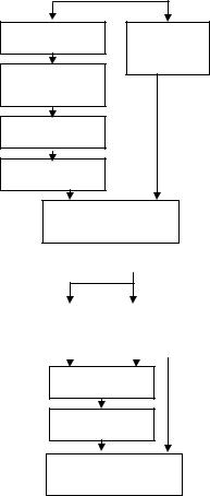
Fig. 6. Video codec diagram Q: Quantizer IQ: Inverse quantizer |
D: Delay |
reduced from the IEEE-standard FP without perceptual quality degradation. In addition, the impacts of other features in IEEE standard, such as the rounding mode, denormalization and the radix choice are also studied. Specifically, we target the IDCT algorithm in a H.263 video codec, since it is the only module that really uses FP computations in the codec, and also is common in many other media applications, such as image processing, audio compression, etc.
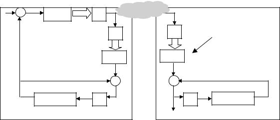
In Fig. 6, we give a simplified diagram of a video codec. In the decoder side, the input compressed video is put into IDCT after inverse quatization. After some FP computations in IDCT, those DCT coefficients are converted to pixel values that are the differences between the previous frame and the current frame. The last step is to get the current frame by adding up the outputs of IDCT and the previous frame after the motion compensation.
Considering the IEEE representation of FP numbers, there are five dimensions that we can explore in order to reduce the hardware complexity (Table 2). Acuracy versus hardware cost trade-off is made in each dimension. In order to measure the accuracy quantitatively, we integrate the Cmufloat IDCT into a
complete video codec and measure the PSNR (Peak-Signal-to- Noise-Ratio) of the decoded video which reflects the decoded vidio quality.
PSNR= 10 log |
2552 |
|
, where N is the total number |
|
N |
|
|||
|
∑ |
( pi − |
f i ) 2 |
|
|
N |
|
|
|
|
i= 0 |
|
|
|
of pixels, pi stands for the pixel value decoded by the lightweight FP algorithm, and fi stands for the reference pixel value of the original video.
4.1Reducing the exponent and fraction bit-width
Reducing the exponent bit-width
The exponent bit-width determines the dynamic range. Using a 5-bit exponent as an example, we derive the dynamic range in Table. 3. Complying with the IEEE standard, the exponent with all 1s is reserved for infinity and NaN. With a bias of 15, the dynamic range for a 5-bit exponent is from 2-14 or 2-15 to 216,
|
Dimension |
|
|
Description |
|
|
|
|
|
|
Smaller exponent bit-width |
|
|
Reduce the number of exponent bits at the expense of dynamic range |
|
|
|
|
|
|
Smaller fraction bit-width |
|
|
Reduce the number of fraction bits at the expense of precision |
|
|
|
|
|
|
Simpler rounding mode |
|
|
Choose simpler rounding mode at the expense of precision |
|
|
|
|
|
|
No support for denormalization |
|
|
Do not support denormalization at the expense of precision |
|
|
|
|
|
|
|
|
|
Increase the implied radix from 2 to 16 for the FP exponent (Higher radix |
|
Higher radix |
|
|
FP needs less exponent bits and more fraction bits than radix-2 FP, in order to |
|
|
|
achieve the comparable dynamic range and precision). |
|
|
|
|
|
|
|
|
|
|
|
Table 2. Working dimensions for lightweight FP
depending on the support for denormalization.
|
|
|
|
|
Exponent |
|
Value of |
|
Dynamic |
|
|
|
|
|
|
|
|
exp - bias |
|
range |
|
|
|
|
|
|
|
|
|
|
||
|
Biggest exponent |
|
11110 |
|
16 |
|
216 |
|
||
|
Smallest |
exponent |
|
|
|
|
|
|
||
|
(with |
support |
for |
00001 |
|
-14 |
|
2-14 |
|
|
|
denrmalization) |
|
|
|
|
|||||
|
|
|
|
|
|
|
|
|||
|
|
|
|
|
|
|
|
|
||
|
Smallest |
exponent |
|
|
|
|
|
|
||
|
(No |
support |
for |
00000 |
|
-15 |
|
2-15 |
|
|
|
denormalization) |
|
|
|
|
|||||
|
|
|
|
|
|
|
|
|||
|
|
|
|
|
|
|||||
|
Table 3. Dynamic range of a 5-bit exponent |
|
|
|||||||
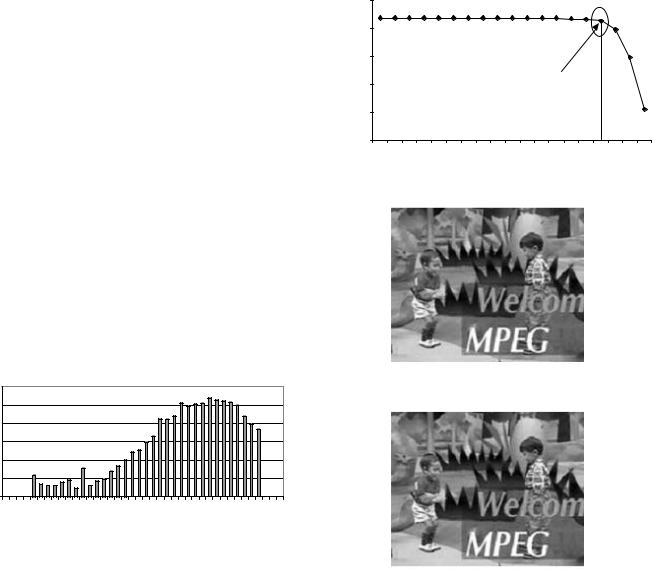
In order to decide the necessary exponent bit-width for our IDCT, we collected the histogram information of exponents for all the variables in the IDCT algorithm during a video sequence decoding (see Fig. 7). The range of these exponents lies in [-22, 10], which is consistent with the theoretical result in [7]. From the dynamic range analysis above, we know that a 5-bit exponent can almost cover such a range except when numbers are extremely small, while a 6-bit exponent can cover the entire range. However, our experiment shows that 5-bit exponent is able to produce the same PSNR as an 8-bit exponent.
1000000
100000
10000
1000
100
10
1
-26 |
-22 |
-18 |
-14 |
-10 |
-6 |
-2 |
2 |
6 |
10 |
Exponent
Fig. 7 Histogram of exponent value
Reducing the fraction bit-width
Reducing the fraction bit-width is the most practical way to lower the hardware cost because the complexity of an integer multiplier is reduced quadratically with decreasing bit-width[19]. On the other hand, the accuracy is degraded when narrowing the bit-width. The influence of decreasing bit-width on video quality is shown in Fig. 8.
As we can see in the curve, PSNR remains almost constant across a rather wide range of fraction bit widths, which means the fraction width does not affect the decoded video quality in this range. The cutoff point where PSNR starts dropping is as small as 8 bits – this is about 1/3 of the fraction-width of an IEEE-standard FP. The difference of PSNR between an 8-bit fraction FP and 23-bit fraction is only 0.22 dB, which is almost not perceptible to human eyes. One frame of the video sequence
|
40 |
|
|
|
|
|
|
|
|
|
|
38 |
|
|
|
|
|
|
|
|
|
PSNR(dB) |
36 |
|
|
|
|
|
|
|
|
|
|
|
|
|
Cutoff point |
|
|
|
|
||
34 |
|
|
|
|
|
|
|
|
|
|
|
|
|
|
|
|
|
|
|
|
|
|
32 |
|
|
|
|
|
|
|
|
|
|
30 |
|
|
|
|
|
|
|
|
|
|
23 |
21 |
19 |
17 |
15 |
13 |
11 |
9 |
7 |
5 |
Fraction width
Fig. 8. PSNR vs. fraction width
Fig. 9 (a) one frame decoded by 32-bit FP 1-bit sign + 8-bit exp + 23-bit fraction
Fig. 9 (b) one frame decoded by 14-bit FP 1-bit sign + 5-bit exp + 8-bit fraction
is compared in Fig. 9. The top one is decoded by a full precision FP IDCT, and the bottom one is decoded by a 14-bit FP IDCT. From the perceptual quality point of view, it’s hard to tell the major difference between these two.
From the above analysis, we can reduce the total bit-width from 32 bits to 14 bits (1-bit sign + 5-bit exponent + 8-bit fraction), while preserving good perceptual quality. In order to generalize our result, the same experiment is carried on three other video sequences: “akiyo”, “stefan”, “mobile”, all of which have around 0.2 dB degradation in PSNR when 14-bit FP is applied.

The relationship between video compression ratio and the minimal bit-width
For streaming video, the lower the bit rate, the worse the video quality. The difference in bit rate is mainly caused by the quantization step size during encoding. A larger step size means coarser quantization and therefore worse video quality. Considering the limited wireless network bandwidth and the low display quality of mobile devices, a relatively low bit rate is preferred to transfer video in this situation. Hence we want to study the relationship between compression ratio, or quantization step size and the minimal bit-width.
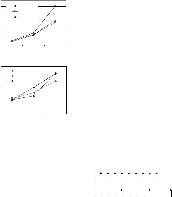
Fig. 10. Comparison of different quantization step
We compare the PSNR curves obtained by experiments with different quantization step sizes in Fig. 10. From the figure, we can see that for a larger quantization step size, the PSNR is lower, but at the same time the curve drops more slowly and the minimal bit-width can be reduced further. This is because coarse quantization can hide more computation error under the quantization noise. Therefore, less computational precision is needed for the video codec using a larger quantization step size.
The relationship between inter/intra coding and the minimal bit-width
Inter coding refers to the coding of each video frame with reference to the previous video frame. That is, only the difference between the current frame and the previous frame is coded, after motion compensation. Since in most videos, adjacent frames are highly correlated, inter coding provides very high efficiency.
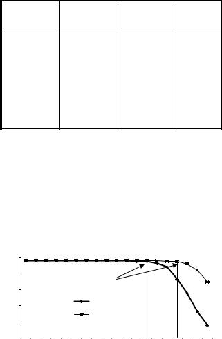
Based on the assumption that video frames have some correlation, for inter-coding, the differences coded as the inputs to DCT are typically much smaller than regular pixel values. Accordingly, the DCT coefficients, or inputs to IDCT are also smaller than those in intra-coding. One property of FP numbers is that representation error is smaller when the number to be represented is smaller. From Fig. 11, the PSNR of inter-coding drops more slowly than intra-coding, or the minimum bit-width of inter-coding can be 1 bit less than intra-coding.
Fig. 11. Comparison of intra-coding and inter-coding
However, if the encoder uses the full precision FP IDCT, while the decoder uses the lightweight FP IDCT, then the error propagation effect of inter-coding can not be eliminated. In that case, inter-coding does not have the above advantage.
The results in this section demonstrates that some programs do not need the extreme precision and dynamic range provided by IEEE-standard FP. Applications dealing with the modestresolution human sensory data can tolerate some computation error in the intermediate or even final results, while giving similar human perceptual results. Some experiments on other applications also agree with this assertion. We also applied Cmufloat to a MP3 decoder. The bit-width can be cut down to 14 bits (1-bit sign + 6-bit exponent + 7-bit fraction) and the noise behind the music is still not perceptible. In the CMU Sphinx application, a speech recognizer, 11-bit FP (1-bit sign + 6-bit exponent + 4-bit fraction) can maintain the same recognition accuracy as 32-bit FP. Such dramatic bit-width reduction offers enormous advantage that may broaden the application of lightweight FP units in mobile devices.
Finally we note that the numerical analysis and precision optimization in this section can be implemented in a semiautomated way by appropriate compiler support. We can extend an existing C++ compiler to handle lightweight arithmetic operations and assist the process of exploring the precision tradeoffs with less programmer intervention. This will unburden designers from translating codes manually into proper limitedprecision formats.
4.2 Rounding modes
When a FP number cannot be represented exactly, or the intermediate result is beyond the allowed bit-width during computation, then the number is rounded, introducing an error less than the value of least significant bit. Among the four rounding modes specified by the IEEE FP standard, round-to- nearest, round-to-(+∞) and round-to-(-∞) need an extra adder in the critical path, while round-toward-zero is the simplest in hardware, but the least accurate in precision. Since round-to- nearest has the most accuracy, we implement it as our baseline of comparison. There is another classical alternative mode that may have potential in both accuracy and hardware cost: Von
Neumann jamming[20]. We will discuss these three rounding modes (round-to-nearest, jamming, round-toward-zero) in detail next.
Round-to-nearest
In the standard FP arithmetic implementation, there are three bits beyond the significant bits that are for intermediate results [9] (see Fig. 12). The sticky bit is the logical OR of all bits thereafter.
significant bit
guard bit
round bit
sticky bit
Fig. 12. guard / round / sticky bit
These three bits participate in rounding in the following way:
b000
b… |
Truncate these tail bits |
|
b011 |
If b is 1, add 1 to b |
|
b100 |
||
If b is 0, truncate the tail bits |
||
b101 |
||
|
||
b… |
Add 1 to b |
|
b111 |
|
Round-to-nearest is the most accurate rounding mode, but needs some comparison logic and a carry-propagate adder in hardware. Further, since the rounding can actually increase the fraction magnitude, it may require extra normalization steps which cause additional fraction and exponent calculations.
Jamming
The rule for Jamming rounding is as follows: if b is 1, then truncate those 3 bits, if b is ‘0’, and there is a ‘1’ among those 3 bits, then add 1 to b, else if b and those 3 bits are all zero, then truncate those 3 bits. Essentially, it is the function of an OR gate (see Fig. 13).
Jamming is extremely simple as hardware – almost as simple as truncation – but numerically more attractive for one subtle but important reason. The rounding created by truncation is biased: the rounded result is always smaller than the correct value. Jamming, by sometimes forcing a ‘1’ into the least significant bit position, is unbiased. The magnitude of Jamming errors is no different from truncation, but the mean of errors is zero. This important distinction was recognized by Von Neuman almost 50 years ago [20].
Round-toward-zero
The operation of round-toward-zero is just truncation. This mode has no overhead in hardware, and it does not have to keep 3 more bits for the intermediate results. So it is much simpler in hardware than the first two modes.
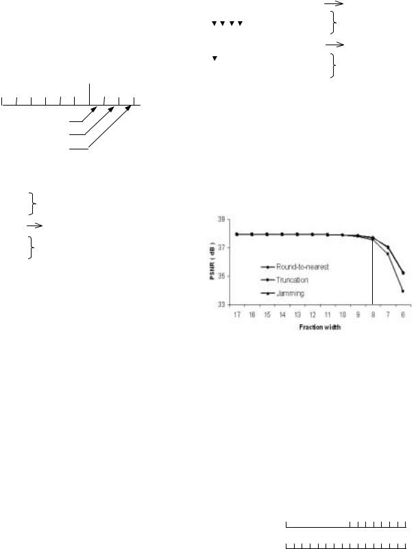
The PNSR curves for the same video sequence obtained using these three rounding modes are shown in Fig. 14. Three
b X X X |
bXXX |
|
||||||
0000 |
Do nothing |
|||||||
|
|
|
|
|
|
|||
|
|
|
|
|
|
0001… |
|
|
|
|
|
|
|
|
0… |
Add 1 to b |
|
|
|
|
|
|
|
|||
|
|
|
|
|
|
|||
|
OR |
|
0111 |
Do nothing |
||||
|
|
|
|
|
|
1000 |
||
|
|
|
|
|
|
|||
|
|
|
|
|
|
1001 |
Truncate tail bits |
|
|
|
|
|
|
|
|||
b’ |
1… |
|||||||
1111 |
|
|||||||
|
|
|
|
|
|
|
||
Fig. 13. Jamming rounding
rounding modes produce almost the same PSNR when the fraction bit-width is more than 8 bits. At the point of 8 bits, the PSNR of truncation is about 0.2 dB worse than the other two. On the other hand, from the hardware point of view, jamming is much simpler than round-to-nearest and truncation is the simplest among these three modes. So tradeoff will be made between quality and complexity among the modes of jamming and truncation. We will finalize the choice of rounding mode during the hardware implementation section.
Fig. 14. Comparison of rounding modes
4.3 Denormalization
The IEEE standard allows for a special set of non-normalized numbers that represent magnitudes very close to zero. We illustrate this in Fig. 15 by an example of a 3-bit fraction. Without denormalization, there is an implicit ‘1’ before the fraction, so the actual smallest fraction is 1.000, while with denormalization, the leading ‘1’ is not enforced so that the smallest fraction is scaled down to 0.001. This mechanism provides more precision for scientific computation with small numbers, but for multimedia applications, especially for video codec, does those small numbers during the computation affect the video quality?
1.000 1.111
Without denormalization
0.001 0.111
With denormalization
Fig. 15. Denormalization
We experimented on the IDCT with a 5-bit exponent Cmufloat representation. 5 bits was chosen to ensure that no overflow happens during the computation. But from the histogram of Fig. 7, there are still some numbers below the threshold of normalized numbers. That means if denormalization is not supported, these numbers will be rounded to zero. However, the experiment shows that the PSNRs with and without denormalization are the same, which means denormalization does not affect the decoded video quality at all.
4.4 Higher radix for FP exponent
The exponent of the IEEE-standard FP is based on radix 2. Historically, there are also systems based on radix 16, for example the IBM 390[10]. The advantage of radix 16 lies mainly in fewer types of shifting during pre-alignment and normalization, which can reduce the shifter complexity in the FP adder and multiplier. We will discuss this issue later when we discuss hardware implementation in more detail.
The potential advantage of a higher radix such as 16 is that the smaller exponent bit-width is needed for the same dynamic range as the radix-2 FP, while the disadvantage is that the larger fraction bit-width has to be chosen to maintain the comparable precision. We analyze such features in the following.
Exponent bit-width
The dynamic range represented by i-bit exponent is |
||
approximately from β 2− ( i − 1) |
to β 2(i − 1) |
( β is the radix). Assume |
we use i-bit exponent for radix-2 FP and j-bit exponent for radix16 FP. If they have the same dynamic range, then 22− ( i − 1) = 162( j − 1) , or j = i-2. Specifically, if the exponent bit-width for radix-2 is 5, then only 3 bits are needed for the radix-16 FP to reach approximately the same range.
Fraction bit-width
The precision of a FP number is mainly determined by the fraction bit-width. But the radix for the exponent also plays a role, due to the way that normalization works. Normalization ensures that no number can be represented two or more bit patterns in the FP format, thus maximizing the use of the finite number of bit patterns. Radix-2 numbers are normalized by shifting to ensure a leading bit ‘1’ in the most significant fraction bit. IEEE format actually makes this implicit, i.e., it is not physically stored in the number.
For radix 16, however, normalization means that the first digit of the fraction, i.e., the most significant 4 bits after the radix point, is never 0000. Hence there are four bit patterns that can appear in the radix-16 fraction (see Table 4). In other words, the radix-16 fraction uses its available bits in a “less efficient” way, because the leading zeros reduce the number of “significant” bits of precision. We analyze the loss of “significant” precisions bits in Table 4.
The significant bit-width of a radix-2 i-bit fraction is i+1, while for a radix-16 j-bit fraction, the significant bit-width is j, j- 1, j-2 or j-3, with possibility of 1/4 respectively. The minimum
fraction bit-width of a radix-16 FP that can guarantee the precision not less than radix-2 must satisfy:
min{ j, j-1, j-2, j-3} ≥ i + 1
, so the minimum fraction bit-width is i + 4. Actually it can provide more precision than radix-2 FP since j, j-1, j-2 are larger than i + 1.
FP format |
Normal |
Range of |
Significant |
|
form of fraction |
fraction |
bits |
|
|
|
|
Radix-2 |
1.xx…xx |
1 ≤ f < 2 |
i + 1 |
|
(i-bit fraction) |
|
|
|
|
|
|
|
|
|
|
.1xx…..x |
1/2 ≤ f < 1 |
j |
|
|
|
|
|
|
Radix-16 |
.01xx…x |
1/4 ≤ f < 1/2 |
j-1 |
|
(j-bit fraction) |
|
|
|
|
.001x…x |
1/8 ≤ f < 1/4 |
j-2 |
||
|
||||
|
|
|
|
|
|
.0001x..x |
1/16 ≤ f < 1/8 |
j-3 |
Table 4. Comparison of radix-2 and radix-16
From previous discussion, we know that 14-bit radix-2 FP (1-bit sign + 5-bit exponent + 8-bit fraction ) can produce good video quality. Moving to radix-16, two less exponent bits (3 bits) and four more fraction bits (12 bits), or 16 bits for total FP can guarantee the comparable video quality. Since the minimum fraction bit-width is derived from the worst-case analysis, it could be reduced further from the perspective of average precision. Applying radix-16 Cmufloat to the video decoder, we can see that the cutoff point actually is 11 bits, not 12 bits for fraction width (Fig. 16 and Table 5 ).
|
40 |
|
|
|
|
|
|
|
|
|
(dB) |
35 |
|
|
|
|
|
|
|
|
|
|
|
|
Cutoff point |
|
|
|
|
|
||
PSNR |
30 |
|
|
|
|
|
|
|
||
|
|
|
|
|
|
|
|
|
||
25 |
|
|
|
R adix 16 |
|
|
|
|
|
|
|
|
|
|
|
|
|
|
|
|
|
|
|
|
|
|
R adix 2 |
|
|
|
|
|
|
20 |
|
|
|
|
|
|
|
|
|
|
15 |
|
|
|
|
|
|
|
|
|
|
2 3 |
2 1 |
1 9 |
1 7 |
15 |
13 |
11 |
9 |
7 |
5 |
Fig. 16. Comparison of radix-2 and radix-16
FP format |
PSNR |
|
|
|
|
Radix-2 |
( 8-bit fraction ) |
38.529 |
|
|
|
Radix-16 |
( 12-bit fraction) |
38.667 |
|
|
|
Radix-16 |
( 11-bit fraction ) |
38.536 |
|
|
|
Radix-16 |
( 10-bit fraction) |
38.007 |
|
|
|
Table 5. 11-bit fraction for radix-16 is sufficient
After discussion in each working dimension, we summarize the lightweight FP design choices for the H.263 video codec in the following:
Data format: 14-bit radx-2 FP (5-bit exponent +8-bit fraction)
or 15-bit radix-16 FP (3-bit exponent + 11-bit fraction) Rounding : Jamming or truncation
Denormalization: Not supported
The final choice of data format and rounding mode are made in the next section according to the hardware cost.
In all discussions in this section, we use PSNR as a measurement of the algorithm. However, we need to mention that there is an IEEE-standard specifying the precision requirement for 8X8 DCT implementation[11]. In the standard, it has the following specification:
7 |
7 |
10000 |
|
|
|
|
∑∑ ∑ek |
2 (i, j) |
|||
omse = |
i= 0 |
j= 0 =k 0 |
|
≤ 0.02 |
|
|
64 × 10000 |
||||
|
|
|
|||
(ek is the pixel difference between reference and proposed IDCT, i and j are the position of the pixel in the 8X8 block)
PSNR specification can be derived from omse: PSNR = 10 log10(2552/omse) ≥ 65.1 dB, which is too tight for videos/images displayed by mobile devices. The other reason we didn’t choose this standard is that it uses the uniform distributed random numbers as input pixels that eliminate the correlation between pixels and enlarge the FP computation error. We also did experiments based on the IEEE-standard. It turns out that around 17-bit fraction is required to meet all the constraints. From PSNR curves in this section, we know that PSNR almost keeps constant for fraction width from 17 bits down to 9 bits. The experimental results support our claim very well that IEEE-standard specifications for IDCT is too strict for encoding/decoding real video sequences.
5. Hardware Implementation of Lightweight FP
Arithmetic Units
FP addition and multiplication are the most frequent FP operations. A lot of work has been published about IEEE compliant FP adders and multipliers, focusing on reducing the latency of the computation. In IBM RISC System/6000, leading- zero-anticipator is introduced in the FP adder [12]. The SNAP project proposed a two-path approach in the FP adder [13]. However, the benefit of these algorithms is not significant and the penalty in area is not ignorable when the bit-width is very small. In this section, we present the structure of the FP adder and multiplier appropriate for narrow bit-width and study the impact of different rounding/exception handling/radix schemes.
Our design is based on Synopsys Designware library and STMicroelectronics 0.18um technology library. The area and latency are measured on gate-level circuit by Synopsys DesignCompiler, and the power consumption is measured by Cadence VerilogXL simulator and Synopsys DesignPower.
Pre-alignment Exception
Detection
Fraction
addition
Normalization
(a) Adder
Rounding
Exception
Handling
Fraction |
|
Exponent |
||||
multipl-cation |
|
addition |
||||
|
|
|
|
|
|
|
Normalization
(b) Multiplier
Rounding
Exception
Handling
Fig. 17. Diagram of FP the adder and multiplier
5.1 Structure
As shown in the diagram (Fig. 17), we take the most straightforward top-level structure for the FP adder and multiplier. The tricks reducing the latency are not adopted because firstly the adder and multiplier can be accelerated easily by pipelining, and secondly those tricks increase the area by a large percentage in the case of narrow bit-width.
Shifter
The core component in the pre-alignment and normalization is a shifter. There are three common architectures for shifter:
N-to-1 Mux shifter is appropriate when N is small.
Logarithmic shifter[14] uses log(N) stages and each stage handles a single, power-of-2 shifts. This architecture has compact area, but the timing path is long when N is big.
Fast two-stage shifter is used in IBM RISC System/6000[15]. The first stage shifts (0, 4, 8, 12,…) bit positions, and the second stage shifts (0, 1, 2, 3) bit position.
The comparison of these three architectures over different bit-widths is shown in Fig. 18. It indicates that for narrow bitwidth (8~16), logarithmic shifter is the best choice considering
both of area and delay, but when the bit-width is increased to a certain level, two-stage shifter become best.
|
|
Area |
|
|
7000 |
|
|
|
6000 |
N-to-1 Mux |
|
|
|
|
|
|
5000 |
Two stages |
|
|
|
|
|
2) |
|
Logrithmic |
|
( um |
4000 |
|
|
|
|
||
|
|
|
|
Area |
3000 |
|
|
|
|
|
|
|
2000 |
|
|
|
1000 |
|
|
|
0 |
|
|
|
8 |
16 |
32 |
Bit width
|
|
Delay |
|
|
6 |
|
|
|
|
N-to-1 Mux |
|
|
5 |
Two stages |
|
|
|
|
|
) |
4 |
Logrithmic |
|
|
|
||
( ns |
3 |
|
|
Delay |
|
|
|
2 |
|
|
|
|
|
|
|
|
1 |
|
|
|
0 |
|
|
|
8 |
16 |
32 |
Bit width
Fig. 18 Area and delay comparisons of three shifter structures
5.2 Rounding
In our lightweight FP arithmetic operations, round-to-nearest is not considered because of the heavy hardware overhead. Jamming rounding demonstrates similar performance as round- to-nearest in the example of video codec. But it still has to keep three more bits in each stage in the FP adder, which becomes significant, especially for narrow bit-width cases. The other candidate is round-toward-zero because its performance is close to Jamming rounding at the cutoff point. Table 6 shows the reduction in both of the area and delay when changing rounding mode from Jamming to round-toward-zero. Since 15% reduction in the area of FP adder can be obtained, we finally choose truncation as the rounding mode.
Rounding mode |
Area (um2) |
Delay (ns) |
|
|
|
Jamming |
7893 |
5.8 |
|
|
|
Truncation |
7741 (-1.9%) |
5.71 (-1.6%) |
|
|
|
Table 6 (a) Comparison of rounding modes–14-bit FP adder
Rounding mode |
Area (um2) |
Delay (ns) |
|
|
|
Jamming |
8401 |
10.21 |
|
|
|
Truncation |
7123 (-15%) |
9.43 (-7.6%) |
|
|
|
Table 6 (b) Comparison of rounding modes–14-bit FP multiplier
5.3 Exception handling
For an IEEE compliant FP arithmetic unit, a large portion of hardware in critical timing path is dedicated for rare exceptional cases, eg. overflow, underflow, infinite, NaN etc. If the exponent bit-width is enough to avoid overflow, then infinite and NaN won’t occur during computation. Then in the FP adder and multiplier diagram (Fig. 17), ‘exception detection’ is not needed and only underflow is detected in ‘exception handling’. As a result, the delay of the FP adder and multiplier is reduced by 9.3% and 20%, respectively, by using partial exception handling.
Exception handling |
Area (um2) |
Delay (ns) |
|
|
|
Full |
8401 |
10.21 |
|
|
|
Partial |
7545 (-10%) |
9.26 (-9.3%) |
|
|
|
Table 7 (a) Comparison of exception handling–14-bit FP adder
Exception handling |
Area (um2) |
Delay (ns) |
|
|
|
|
|
Full |
7893 |
|
5.8 |
|
|
|
|
Partial |
7508 |
(-4.9%) |
4.62 (-20%) |
|
|
|
|
Table7 (b) Comparison of exception handling-14-bit multiplier
5.4 Radix
The advantage of higher radix FP is less complexity in the shifter. From section 4, we know that in video codec, the precision of radix-16 FP with 11-bit fraction is close to radix-2 FP with 8-bit fraction. We illustrate the difference in shifter in Fig. 19. The step size of shifting for radix-16 is four and only three shifting positions are needed. Such a simple shifter can be implemented by the structure of 3-to-1 Mux. Although there are 3 more bits in the fraction, FP adder still benefited from higher radix in both area and delay (Table 8).
(a ) Radix-2 FP ( 8-bit fraction + 1 leading bit )
(b) Radix-16 FP ( 11-bit fraction ) |
Fig. 19 Shifting positions for radix-2 and radix-16 FP
On the other hand, more fraction width increases the complexity of the FP multiplier. The size of multiplier is increased about quadratically with the bit-width, so only 3 more bits can increase the multiplier’s area by 43% (Table 8).