
7
Design and Performance
7.1 INTRODUCTION
The MPEG-4 Visual and H.264 standards include a range of coding tools and processes and there is significant scope for differences in the way standards-compliant encoders and decoders are developed. Achieving good performance in a practical implementation requires careful design and careful choice of coding parameters.
In this chapter we give an overview of practical issues related to the design of software or hardware implementations of the coding standards. The design of each of the main functional blocks of a CODEC (such as motion estimation, transform and entropy coding) can have a significant impact on computational efficiency and compression performance. We discuss the interfaces to a video encoder and decoder and the value of video pre-processing to reduce input noise and post-processing to minimise coding artefacts.
Comparing the performance of video coding algorithms is a difficult task, not least because decoded video quality is dependent on the input video material and is inherently subjective. We compare the subjective and objective (PSNR) coding performance of MPEG-4 Visual and H.264 reference model encoders using selected test video sequences. Compression performance often comes at a computational cost and we discuss the computational performance requirements of the two standards.
The compressed video data produced by an encoder is typically stored or transmitted across a network. In many practical applications, it is necessary to control the bitrate of the encoded data stream in order to match the available bitrate of a delivery mechanism. We discuss practical bitrate control and network transport issues.
7.2 FUNCTIONAL DESIGN
Figures 3.51 and 3.52 show typical structures for a motion-compensated transform based video encoder and decoder. A practical MPEG-4 Visual or H.264 CODEC is required to implement some or all of the functions shown in these figures (even if the CODEC structure is different
H.264 and MPEG-4 Video Compression: Video Coding for Next-generation Multimedia.
Iain E. G. Richardson. C 2003 John Wiley & Sons, Ltd. ISBN: 0-470-84837-5

• |
DESIGN AND PERFORMANCE |
226 |
from that shown). Conforming to the MPEG-4/H.264 standards, whilst maintaining good compression and computational performance, requires careful design of the CODEC functional blocks. The goal of a functional block design is to achieve good rate/distortion performance (see Section 7.4.3) whilst keeping computational overheads to an acceptable level.
Functions such as motion estimation, transforms and entropy coding can be highly computationally intensive. Many practical platforms for video compression are power-limited or computation-limited and so it is important to design the functional blocks with these limitations in mind. In this section we discuss practical approaches and tradeoffs in the design of the main functional blocks of a video CODEC.
7.2.1 Segmentation
The object-based functionalities of MPEG-4 (Core, Main and related profiles) require a video scene to be segmented into objects. Segmentation methods usually fall into three categories:
1.Manual segmentation: this requires a human operator to identify manually the borders of each object in each source video frame, a very time-consuming process that is obviously only suitable for ‘offline’ video content (video data captured in advance of coding and transmission). This approach may be appropriate, for example, for segmentation of an important visual object that may be viewed by many users and/or re-used many times in different composed video sequences.
2.Semi-automatic segmentation: a human operator identifies objects and perhaps object boundaries in one frame; a segmentation algorithm refines the object boundaries (if necessary) and tracks the video objects through successive frames of the sequence.
3.Fully-automatic segmentation: an algorithm attempts to carry out a complete segmentation of a visual scene without any user input, based on (for example) spatial characteristics such as edges and temporal characteristics such as object motion between frames.
Semi-automatic segmentation [1,2] has the potential to give better results than fully-automatic segmentation but still requires user input. Many algorithms have been proposed for automatic segmentation [3,4]. In general, better segmentation performance can be achieved at the expense of greater computational complexity. Some of the more sophisticated segmentation algorithms require significantly more computation than the video encoding process itself. Reasonably accurate segmentation performance can be achieved by spatio-temporal approaches (e.g. [3]) in which a coarse approximate segmentation is formed based on spatial information and is then refined as objects move. Excellent segmentation results can be obtained in controlled environments (for example, if a TV presenter stands in front of a blue background) but the results for practical scenarios are less robust.
The output of a segmentation process is a sequence of mask frames for each VO, each frame containing a binary mask for one VOP (e.g. Figure 5.30) that determines the processing of MBs and blocks and is coded as a BAB in each boundary MB position.
7.2.2 Motion Estimation
Motion estimation is the process of selecting an offset to a suitable reference area in a previously coded frame (see Chapter 3). Motion estimation is carried out in a video encoder (not in a

32×32 block in current frame
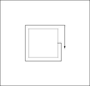
Figure 7.1 Current block (white border)
decoder) and has a significant effect on CODEC performance. A good choice of prediction reference minimises the energy in the motion-compensated residual which in turn maximises compression performance. However, finding the ‘best’ offset can be a very computationallyintensive procedure.
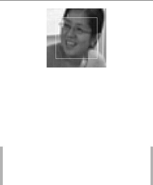
The offset between the current region or block and the reference area (motion vector) may be constrained by the semantics of the coding standard. Typically, the reference area is constrained to lie within a rectangle centred upon the position of the current block or region. Figure 7.1 shows a 32 × 32-sample block (outlined in white) that is to be motion-compensated. Figure 7.2 shows the same block position in the previous frame (outlined in white) and a larger square extending ± 7 samples around the block position in each direction. The motion vector may ‘point’ to any reference area within the larger square (the search area). The goal of a practical motion estimation algorithm is to find a vector that minimises the residual energy after motion compensation, whilst keeping the computational complexity within acceptable limits. The choice of algorithm depends on the platform (e.g. software or hardware) and on whether motion estimation is block-based or region-based.
7.2.2.1 Block Based Motion Estimation
Energy Measures
Motion compensation aims to minimise the energy of the residual transform coefficients after quantisation. The energy in a transformed block depends on the energy in the residual block (prior to the transform). Motion estimation therefore aims to find a ‘match’ to the current block or region that minimises the energy in the motion compensated residual (the difference between the current block and the reference area). This usually involves evaluating the residual energy at a number of different offsets. The choice of measure for ‘energy’ affects computational complexity and the accuracy of the motion estimation process. Equation 7.1, equation 7.2 and equation 7.3 describe three energy measures, MSE, MAE and SAE. The motion
228 |
DESIGN AND PERFORMANCE |
• |
Previous (reference) frame |
Figure 7.2 Search region in previous (reference) frame
compensation block size is N × N samples; Ci j and Ri j are current and reference area samples respectively.
|
|
1 |
N −1 N −1 |
|
|
|
|
|
|
|
1. |
Mean Squared Error: |
M S E = |
N 2 |
(Ci j − Ri j )2 |
(7.1) |
|
|
|
|
i =0 j =0 |
|
|
|
1 |
N −1 N −1 |
|
2. |
Mean Absolute Error: |
M AE = |
|
|
(7.2) |
N 2 |
|Ci j − Ri j | |
|
|
|
|
i =0 j =0 |
|
|
|
N −1 N −1 |
|
3. |
Sum of Absolute Errors: |
|
(7.3) |
S AE = |
|Ci j − Ri j | |
|
|
|
i =0 |
j =0 |
|
Example
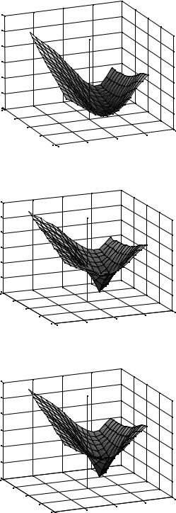
Evaluating MSE for every possible offset in the search region of Figure 7.2 gives a ‘map’ of MSE (Figure 7.3). This graph has a minimum at (+2, 0) which means that the best match is obtained by selecting a 32 × 32 sample reference region at an offset of 2 to the right of the block position in the current frame. MAE and SAE (sometimes referred to as SAD, Sum of Absolute Differences) are easier to calculate than MSE; their ‘maps’ are shown in Figure 7.4 and Figure 7.5. Whilst the gradient of the map is different from the MSE case, both these measures have a minimum at location (+2, 0).
SAE is probably the most widely-used measure of residual energy for reasons of computational simplicity. The H.264 reference model software [5] uses SA(T)D, the sum of absolute differences of the transformed residual data, as its prediction energy measure (for both Intra and Inter prediction). Transforming the residual at each search location increases computation but improves the accuracy of the energy measure. A simple multiply-free transform is used and so the extra computational cost is not excessive.
The results of the above example indicate that the best choice of motion vector is (+2,0). The minimum of the MSE or SAE map indicates the offset that produces a minimal residual energy and this is likely to produce the smallest energy of quantised transform
• |
DESIGN AND PERFORMANCE |
230 |
Search ‘window’
Initial search |
location |
Raster search order |
Centre (0,0)
position
Figure 7.6 Full search (raster scan)
coefficients. The motion vector itself must be transmitted to the decoder, however, and as larger vectors are coded using more bits than small-magnitude vectors (see Chapter 3) it may be useful to ‘bias’ the choice of vector towards (0,0). This can be achieved simply by subtracting a constant from the MSE or SAE at position (0,0). A more sophisticated approach is to treat the choice of vector as a constrained optimisation problem [6]. The H.264 reference model encoder [5] adds a cost parameter for each coded element (MVD, prediction mode, etc) before choosing the smallest total cost of motion prediction.
It may not always be necessary to calculate SAE (or MAE or MSE) completely at each offset location. A popular shortcut is to terminate the calculation early once the previous minimum SAE has been exceeded. For example, after calculating each inner sum of equation (7.3)
|
N −1 |
|Ci j − Ri j |), the encoder compares the total SAE with the previous minimum. If the |
( j =0 |
total so far exceeds the previous minimum, the calculation is terminated (since there is no point in finishing the calculation if the outcome is already higher than the previous minimum SAE).
Full Search
Full Search motion estimation involves evaluating equation 7.3 (SAE) at each point in the search window (±S samples about position (0,0), the position of the current macroblock). Full search estimation is guaranteed to find the minimum SAE (or MAE or MSE) in the search window but it is computationally intensive since the energy measure (e.g. equation (7.3)) must be calculated at every one of (2S + 1)2 locations.
Figure 7.6 shows an example of a Full Search strategy. The first search location is at the top-left of the window (position [−S, −S]) and the search proceeds in raster order
Search ‘window’
Initial search |
location |
Spiral |
search |
order |
Figure 7.7 Full search (spiral scan)
until all positions have been evaluated. In a typical video sequence, most motion vectors are concentrated around (0,0) and so it is likely that a minimum will be found in this region. The computation of the full search algorithm can be simplified by starting the search at (0,0) and proceeding to test points in a spiral pattern around this location (Figure 7.7). If early termination is used (see above), the SAE calculation is increasingly likely to be terminated early (thereby saving computation) as the search pattern widens outwards.
‘Fast’ Search Algorithms
Even with the use of early termination, Full Search motion estimation is too computationally intensive for many practical applications. In computationor power-limited applications, socalled ‘fast search’ algorithms are preferable. These algorithms operate by calculating the energy measure (e.g. SAE) at a subset of locations within the search window.
The popular Three Step Search (TSS, sometimes described as N-Step Search) is illustrated in Figure 7.8. SAE is calculated at position (0,0) (the centre of the Figure) and at eight locations
±2N −1 (for a search window of ±(2N − 1) samples). In the figure, S is 7 and the first nine search locations are numbered ‘1’. The search location that gives the smallest SAE is chosen as the new search centre and a further eight locations are searched, this time at half the previous distance from the search centre (numbered ‘2’ in the figure). Once again, the ‘best’ location is chosen as the new search origin and the algorithm is repeated until the search distance cannot be subdivided further. The TSS is considerably simpler than Full Search (8N + 1 searches compared with (2N +1 − 1)2 searches for Full Search) but the TSS (and other fast
232 |
|
|
|
|
DESIGN AND PERFORMANCE |
• |
2 |
|
2 |
2 |
|
1 |
2 |
|
1 |
2 |
1 |
3 |
3 |
3 |
|
|
|
3 |
2 |
3 |
2 |
2 |
|
3 |
3 |
3 |
|
|
|
1 |
|
|
1 |
|
1 |
Figure 7.8 Three Step Search
0
Figure 7.9 SAE map showing several local minima
search algorithms) do not usually perform as well as Full Search. The SAE map shown in Figure 7.5 has a single minimum point and the TSS is likely to find this minimum correctly, but the SAE map for a block containing complex detail and/or different moving components may have several local minima (e.g. see Figure 7.9). Whilst the Full Search will always identify the global minimum, a fast search algorithm may become ‘trapped’ in a local minimum, giving a suboptimal result.

|
3 |
2 |
|
3 |
2 |
1 |
2 |
|
1 |
1 |
1 |
|
|
1 |
Predicted vector |
|
|
|
0 |
Figure 7.10 Nearest Neighbours Search
Many fast search algorithms have been proposed, such as Logarithmic Search, Hierarchical Search, Cross Search and One at a Time Search [7–9]. In each case, the performance of the algorithm can be evaluated by comparison with Full Search. Suitable comparison criteria are compression performance (how effective is the algorithm at minimising the motion-compensated residual?) and computational performance (how much computation is saved compared with Full Search?). Other criteria may be helpful; for example, some ‘fast’ algorithms such as Hierarchical Search are better-suited to hardware implementation than others.
Nearest Neighbours Search [10] is a fast motion estimation algorithm that has low computational complexity but closely approaches the performance of Full Search within the framework of MPEG-4 Simple Profile. In MPEG-4 Visual, each block or macroblock motion vector is differentially encoded. A predicted vector is calculated (based on previously-coded vectors from neighbouring blocks) and the difference (MVD) between the current vector and the predicted vector is transmitted. NNS exploits this property by giving preference to vectors that are close to the predicted vector (and hence minimise MVD). First, SAE is evaluated at location (0,0). Then, the search origin is set to the predicted vector location and surrounding points in a diamond shape are evaluated (labelled ‘1’ in Figure 7.10). The next step depends on which of the points have the lowest SAE. If the (0,0) point or the centre of the diamond have the lowest SAE, then the search terminates. If a point on the edge of the diamond has the lowest SAE (the highlighted point in this example), that becomes the centre of a new diamond-shaped search pattern and the search continues. In the figure, the search terminates after the points marked ‘3’ are searched. The inherent bias towards the predicted vector gives excellent compression performance (close to the performance achieved by full search) with low computational complexity.
Sub-pixel Motion Estimation
Chapter 3 demonstrated that better motion compensation can be achieved by allowing the offset into the reference frame (the motion vector) to take fractional values rather than just integer values. For example, the woman’s head will not necessarily move by an integer number of pixels from the previous frame (Figure 7.2) to the current frame (Figure 7.1). Increased
• |
DESIGN AND PERFORMANCE |
234 |
fractional accuracy (half-pixel vectors in MPEG-4 Simple Profile, quarter-pixel vectors in Advanced Simple profile and H.264) can provide a better match and reduce the energy in the motion-compensated residual. This gain is offset against the need to transmit fractional motion vectors (which increases the number of bits required to represent motion vectors) and the increased complexity of sub-pixel motion estimation and compensation.
Sub-pixel motion estimation requires the encoder to interpolate between integer sample positions in the reference frame as discussed in Chapter 3. Interpolation is computationally intensive, especially so for quarter-pixel interpolation because a high-order interpolation filter is required for good compression performance (see Chapter 6). Calculating sub-pixel samples for the entire search window is not usually necessary. Instead, it is sufficient to find the best integer-pixel match (using Full Search or one of the fast search algorithms discussed above) and then to search interpolated positions adjacent to this position. In the case of quarter-pixel motion estimation, first the best integer match is found; then the best half-pixel position match in the immediate neighbourhood is calculated; finally the best quarter-pixel match around this half-pixel position is found.
7.2.2.2 Object Based Motion Estimation
Chapter 5 described the process of motion compensated prediction and reconstruction (MC/MR) of boundary MBs in an MPEG-4 Core Profile VOP. During MC/MR, transparent pixels in boundary and transparent MBs are padded prior to forming a motion compensated prediction. In order to find the optimum prediction for each MB, motion estimation should be carried out using the padded reference frame. Object-based motion estimation consists of the following steps.
1.Pad transparent pixel positions in the reference VOP as described in Chapter 5.
2.Carry out block-based motion estimation to find the best match for the current MB in the padded reference VOP. If the current MB is a boundary MB, the energy measure should only be calculated for opaque pixel positions in the current MB.
Motion estimation for arbitrary-shaped VOs is more complex than for rectangular frames (or slices/VOs). In [11] the computation and compression performance of a number of popular motion estimation algorithms are compared for the rectangular and object-based cases. Methods of padding boundary MBs using graphics co-processor functions are described in [12] and a hardware architecture for Motion Estimation, Motion Compensation and CAE shape coding is presented in [13].
7.2.3 DCT/IDCT
The Discrete Cosine Transform is widely used in image and video compression algorithms in order to decorrelate image or residual data prior to quantisation and compression (see Chapter 3). The basic FDCT and IDCT equations (equations (3.4) and (3.5)), if implemented directly, require a large number of multiplications and additions. It is possible to exploit the structure of the transform matrix A in order to significantly reduce computational complexity and this is one of the reasons for the popularity of the DCT.
7.2.3.1 8 × 8 DCT
Direct evaluation of equation (3.4) for an 8 × 8 FDCT (where N = 8) requires 64 × 64 = 4096 multiplications and accumulations. From the matrix form (equation (3.1)) it is clear that the 2D transform can be evaluated in two stages (i.e. calculate AX and then multiply by matrix AT, or vice versa). The 1D FDCT is given by equation (7.4), where fi are the N input samples and Fx are the N output coefficients. Rearranging the 2D FDCT equation (equation (3.4)) shows that the 2D FDCT can be constructed from two 1D transforms (equation (7.5)). The 2D FDCT may be calculated by evaluating a 1D FDCT of each column of the input matrix (the inner transform), then evaluating a 1D FDCT of each row of the result of the first set of transforms (the outer transform). The 2D IDCT can be manipulated in a similar way (equation (7.6)). Each eight-point 1D transform takes 64 multiply/accumulate operations, giving a total of 64 × 8 × 2 = 1024 multiply/accumulate operations for an 8 × 8 FDCT or IDCT.
|
|
|
|
|
|
|
|
F |
|
|
|
C |
N −1 |
f |
|
cos (2i + 1)xπ |
|
|
(7.4) |
|
|
|
|
|
|
|
|
x |
|
= x |
|
|
i |
|
|
|
|
|
|
|
|
|
|
|
|
|
|
|
|
|
|
|
|
|
|
|
|
|
|
2N |
|
|
|
|
|
|
|
x y = |
|
|
|
|
|
|
|
|
|
|
|
i =0 |
|
|
|
|
|
|
|
|
|
|
|
|
|
|
x |
i 0 |
|
y |
|
j 0 |
|
|
i j |
|
|
|
|
|
2N |
|
|
2N |
|
|
|
|
|
|
N −1 |
|
|
|
N −1 |
|
|
|
|
|
|
|
(2 j |
1)yπ |
|
|
|
(2i |
1)xπ |
|
Y |
|
|
C |
|
|
|
C |
|
|
|
X |
|
cos |
|
+ |
|
cos |
+ |
|
(7.5) |
|
|
|
|
= |
|
|
|
= |
|
|
|
|
|
|
|
|
|
i j = x 0 |
|
y 0 |
|
|
|
|
|
|
|
|
|
|
|
|
|
|
|
|
|
X |
|
x |
|
y |
Y |
x y |
cos |
|
|
2N |
|
|
2N |
(7.6) |
|
N |
−1 C |
|
N |
−1 C |
|
|
(2 j + |
1)yπ |
cos (2i + |
1)xπ |
|
|
|
|
|
|
|
|
|
|
|
|
|
|
|
|
|
|
|
|
|
|
|
|
|
|
|
|
= |
|
|
|
|
= |
|
|
|
|
|
|
|
|
|
|
|
|
|
|
|
|
|
|
|
At first glance, calculating an eight-point 1-D FDCT (equation (7.4)) requires the evaluation of
eight different cosine factors (cos (2i +1)xπ with eight values of i ) for each of eight coefficient
2N
indices (x = 0 . . . 7). However, the symmetries of the cosine function make it possible to combine many of these calculations into a reduced number of steps. For example, consider the calculation of F2 (from equation (7.4)):
F2 = |
2 |
f0 |
|
8 |
|
+ f1 cos |
8 |
|
+ f2 cos |
8 |
|
+ f3 cos |
8 |
+ f4 cos |
8 |
|
|
1 |
|
|
π |
|
|
|
|
3π |
|
|
|
5π |
|
|
|
7π |
|
9π |
|
|
|
|
|
|
|
|
|
|
|
|
|
|
|
|
|
|
|
|
|
|
|
+ f5 cos |
8 |
+ f6 cos |
8 |
+ f7 cos |
8 |
|
|
(7.7) |
|
|
|
|
|
|
|
11π |
|
|
|
|
13π |
|
|
|
|
15π |
|
|
|
|
|
Evaluating equation (7.7) would seem to require eight multiplications and seven additions (plus a scaling by a half). However, by making use of the symmetrical properties of the cosine function this can be simplified to:
F2 |
= |
2 |
( f0 |
− f4 |
+ f7 |
− f3). cos |
|
8 |
|
+ ( f1 − f2 − f5 + f6). cos |
8 |
|
(7.8) |
|
|
1 |
|
|
|
|
|
π |
|
|
|
3π |
|
|
In a similar way, F6 may be simplified to: |
|
8 |
|
+ ( f1 − f2 − f5 + f6). cos |
|
8 |
|
(7.9) |
F6 |
= |
2 |
( f0 |
− f4 |
+ f7 |
− f3). cos |
|
|
|
1 |
|
|
|
|
|
3π |
|
|
π |
|
|
The additions and subtractions are common to both coefficients and need only be carried out once so that F2 and F6 can be calculated using a total of eight additions and four multiplications (plus a final scaling by a half). Extending this approach to the complete 8 × 8 FDCT leads to a number of alternative ‘fast’ implementations such as the popular algorithm due to
236 |
|
|
|
DESIGN AND PERFORMANCE |
•f0 |
|
|
c4 |
c4 |
2F0 |
f1 |
|
|
|
c4 |
2F4 |
|
|
-c4 |
|
f2 |
|
-1 |
c6 |
|
2F2 |
|
|
|
|
c2 |
|
f3 |
|
-1 |
|
-c2 |
2F6 |
|
c6 |
|
f4 |
-1 |
|
|
c7 |
2F1 |
|
|
|
|
|
c1 |
f5 |
-1 |
-c4 |
-1 |
c3 |
2F5 |
|
|
c4 |
|
|
c5 |
|
|
c4 |
|
|
-c5 |
f6 |
-1 |
c4 |
-1 |
c3 |
2F3 |
|
|
|
|
|
-c1 |
f7 |
-1 |
|
|
c7 |
2F7 |
Figure 7.11 FDCT flowgraph
Chen, Smith and Fralick [14]. The data flow through this 1D algorithm can be represented as a ‘flowgraph’ (Figure 7.11). In this figure, a circle indicates addition of two inputs, a square indicates multiplication by a constant and cX indicates the constant cos(X π/16). This algorithm requires only 26 additions or subtractions and 20 multiplications (in comparison with the 64 multiplications and 64 additions required to evaluate equation (7.4)).
Figure 7.11 is just one possible simplification of the 1D DCT algorithm. Many flowgraphtype algorithms have been developed over the years, optimised for a range of implementation requirements (e.g. minimal multiplications, minimal subtractions, etc.) Further computational gains can be obtained by direct optimisation of the 2D DCT (usually at the expense of increased implementation complexity).
Flowgraph algorithms are very popular for software CODECs where (in many cases) the best performance is achieved by minimising the number of computationally-expensive multiply operations. For a hardware implementation, regular data flow may be more important than the number of operations and so a different approach may be required. Popular hardware architectures for the FDCT / IDCT include those based on parallel multiplier arrays and distributed arithmetic [15–18].
7.2.3.2 H.264 4 × 4 Transform
The integer IDCT approximations specified in the H.264 standard have been designed to be suitable for fast, efficient software and hardware implementation. The original proposal for the
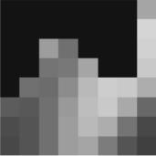
Figure 7.12 8 × 8 block in boundary MB
forward and inverse transforms [19] describes alternative implementations using (i) a series of shifts and additions (‘shift and add’), (ii) a flowgraph algorithm and (iii) matrix multiplications. Some platforms (for example DSPs) are better-suited to ‘multiply-accumulate’ calculations than to ‘shift and add’ operations and so the matrix implementation (described in C code in [20]) may be more appropriate for these platforms.
7.2.3.3 Object Boundaries
In a Core or Main Profile MPEG-4 CODEC, residual coefficients in a boundary MB are coded using the 8 × 8 DCT. Figure 7.12 shows one block from a boundary MB (with the transparent pixels set to 0 and displayed here as black). The entire block (including the transparent pixels) is transformed with an 8 × 8 DCT and quantised and the reconstructed block after rescaling and inverse DCT is shown in Figure 7.13. Note that some of the formerly transparent pixels are now nonzero due to quantisation distortion (e.g. the pixel marked with a white ‘cross’). The decoder discards the transparent pixels (according to the BAB transparency map) and retains the opaque pixels.
Using an 8 × 8 DCT and IDCT for an irregular-shaped region of opaque pixels is not ideal because the transparent pixels contribute to the energy in the DCT coefficients and so more data is coded than is absolutely necessary. Because the transparent pixel positions are discarded by the decoder, the encoder may place any data at all in these positions prior to the DCT. Various strategies have been proposed for filling (padding) the transparent positions prior to applying the 8 × 8 DCT, for example, by padding with values selected to minimise the energy in the DCT coefficients [21, 22], but choosing the optimal padding values is a computationally expensive process. A simple alternative is to pad the transparent positions in an inter-coded MB with zeros (since the motion-compensated residual is usually close to zero anyway) and to pad the transparent positions in an inter-coded MB with the value 2N −1, where N is the number of bits per pixel (since this is mid-way between the minimum and maximum pixel value). The Shape-Adaptive DCT (see Chapter 5) provides a more efficient solution for transforming irregular-shaped blocks but is computationally intensive and is only available in the Advanced Coding Efficiency Profile of MPEG-4 Visual.


 -10
-10

