74	CHAPTER 3. FERMIONS

It turns out that the region of temperatures dT around TC where fluctuations become important can be estimated as

4

dT TC eF (3.238)

This is so small that it cannot be found experimentally.

3.5.2 BCS Hamiltonian

The goal is to modify the HAMILTONian (3.111) in such a way that the BCS relevant terms are clearly visible while other terms (which are not relevant in this context) are put aside. We assume two types of FERMIonswhich we will denote as + and . In this case the interaction part of (3.111) can be written as3

ˆ	0	† †
Hint	= V0å	ap3+ap4 ap2 ap1+	(3.239)
	pi

We are not interested here in the FERMI-liquid type of renormalisations due to the interaction but only for the terms responsible for the COOPER coupling. Since we neglect all other terms we can write

ˆ = ån + † † o+

Hint a p ap+ ap+ap other terms (3.240)

p

We approximate the operator by its mean field value and note, that the first term

destroys a COOPER pair while the second term creates a COOPER pair.	has to
be calculated as
= jV0jåha p ap+i	(3.241)
p

This is a HARTREE-FOCK type of equation, i.e. (3.240) and (3.241) have to be solved self-consistently.

We can choose real since a space independent phase would be irrelevant and a space dependent phase would cause a probability flow but we are looking for a stationary ground state solution. Thus we have

Hˆ eff = åp j xpa†p jap j åp					na p ap+ + a†p+a†		p o	(3.242)
	p2			p2
xp =		m	m =		F			(3.243)
	2m			2m

3for simplicity we now always write p instead of ~p

3.5. BARDEEN-COOPER-SHIEFFER-THEORY

75

This case is different to the one encountered in section (2.3) because here we have

	ˆ
to calculate H and simultaneously.
Again we can make a BOGOLYUBOV transformation							† p
ap j	= upa˜ p j	+ sign( j)vpa˜ †	p j = (ap+ = upa˜ p+			vpa˜		j =		(3.244)
			˜			˜	†	j = +
			ap = upap		+ vpa
							p+
The transformation has to be canonical, thus
		na˜ p j;a˜ p0 j0o = na˜ †p j;a˜ †p0 j0o = 0								(3.245)

no

˜	˜ †	= dpp0dj j0	(3.246)
ap j	;ap0 j0

We again assume the most simple arrangement, i.e.

up = up	vp = vp	(3.247)
and insert the new operators in the FERMI anticommutating relations:
nap j;ap0 j0o = na†p j;a†p0 j0o = 0		(3.248)

no

a

p j

;a

†

j0

u

˜

˜

a˜

j;

(3.249)

p0

a˜ †

+ sign( j0)v

=

upap j

+ sign( j)vpa

p

= upup0dpp0dj j0 + sign( j)sign( j0)vpvp0dpp0dj j0

(3.250)

p

p0

j0

p0

p0

j0

= d

d

j j0

(u2

+ v2 )

(3.251)

pp0

p

p

Thus we have the requirement that

u2p + v2p = 1;

(3.252)

which means that up and vp have to be expressed as sine and cosine. Finally the transformed HAMILTONian has to have the following form

ˆ	˜ † ˜	(3.253)
Heff	= E0 + åepap jap j

p j

The coefficients up and vp can be calculated from the dynamics of the system. To this end we calculate

hHˆ eff;a˜ p ji = på0 j0	ep0		a˜ †p0 j0a˜ p0 j0a˜ p j a˜ p ja˜ †p0 j0a˜ p0 j0							(3.254)
= på0 j0		ep0			a˜ †p0 j0a˜ p j	+	a˜ p ja˜ †p0 j0	a˜ p0 j0		(3.255)
= epa˜ p j				|	=d	p{zp0	dj j0	}		(3.256)

76	CHAPTER 3. FERMIONS

The other commutator we do not need to calculate because

hHˆ eff;a˜ †p ji = hHˆ eff;a˜ p ji†				= epa˜ †p j
Now let’s use this to calculate the commutator
hHˆ eff;ap ji = hHˆ eff;upa˜ p j + sign( j)vpa˜ †			p† ji
˜		˜
= up( ep)ap j + sign( j)vpepa p j					p0
=! xpap j åp0	a†p0+a†	p0 ap j ap ja†p0+a†
= xpap j åp0	a†p0+a†	p0 ap j

d

pp

0

d

j+

a†

+

a

†

a†

0

† 0

p

p j

p

= xpap j åp0

nap0+a p0 ap j

dpp0dj+a†	p0 †	+ a†p0+ dp † p0dj
= xpap j + dj+a p dj a p+
= xpap j + sign( j)a†			p j	p j
= xp upa˜ p j + sign( j)vpa˜ †

o

a† p0 ap j

(3.257)

(3.258)

(3.259)

(3.260)

(3.261)

(3.262)

(3.263)

(3.264)

+ sign( j) upa˜ † p j + sign( j)vpa˜ p j (3.265)

Conferring to (3.259) we get the BOGOLYUBOV-DE GENNES equations:

			epup = xpup vp							(3.266)
			epvp = xpvp + up							(3.267)
which are solved by
ep = q
			2 + xp2			v2p =	2	1 ep		(3.268)
u2p =	2	1 + ep								(3.269)
	1			xp			1	xp

The solution is very similar to the BOSE case.

It follows from (3.268) that ep is always positive, ep > 0.

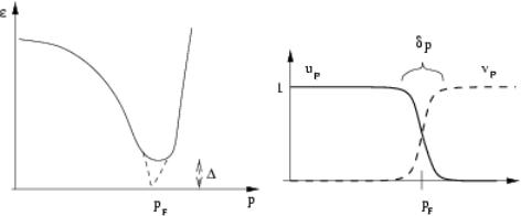
The pairing energy is eF which causes the edges of the FERMI sphere to smear out. The BCS gap in the spectrum can be experimentally observed because

3.5. BARDEEN-COOPER-SHIEFFER-THEORY

77

Figure 3.5: Spectrum of FERMIons with COOPER pairing (left) and plot of u and v as a function of p

the medium is transparent for all external perturbations with frequency w < 2

which couple to single particle excitations.

We now want to calculate

:

p i

= jV0jåp h upa˜ p vpa˜ †p+ upa˜ p+ + vpa˜ †

(3.270)

= jV0jåp

upvp ha˜ p a˜ †

p i ha˜ †p+a˜ p+i

(3.271)

= jV0jåupvp(1 2np)

(3.272)

p

= V0

å 1 q

tanh

ep

=

V0

å tanh

2T

(3.273)

ep2 xp2

ep

j

j

j

j

p 2

ep

2T

p

2ep

where we used

np

=

˜ †

˜

=

˜

†

˜

=

1

(3.274)

p

p

e

ap+ap+

a

a

h

i

h

i

exp

p

+ 1

T

which is the number of particles involved. Thus we have

tanh		ep		ep = q
		2T
1 = jV0jåp					2 + xp2	(3.275)
	2ep

This equation determines (T ). We are mainly interested in the gap near TC, i.e.

1 = V0		å tanh			2TC	(3.276)
					xp
j	j
		p	2xp

78	CHAPTER 3. FERMIONS

which might become problematic for xp ! 0. To solve this, we have to use the scattering length analogous to (3.125) and rewrite the expression as

1 = 4p~ j j å

8

h

C i

p2

9

tanh

xp

1

m

2 a

<

2T

=

p

2xp

2

2m

∞:

;

2T

=

4p~ jaj

dx n(x + eF)

8

h

C i

m

x

2

Z eF

<

tanh

2xp

:

			(3.277)
	2(x + eF)	=
	1	9	(3.278)

;

2

8

h

p2 pF2

i

9

=

4p~

jaj

d p p2

C

1

2 3

p

2

p

2

2

m

m

∞

p

2p ~

Z0

<

F

=

= l

∞

dx x

2

tanh a(x2

:1)

1

;

0

(

x2

1

x2 )

= l

Z

1

)

0

dx (tanh a(x2 1) 1 +

tanh

x2

1)

∞

a

(x2

Z

Z

= ln x

tanh

a(x2 1)

1

∞

2ax

0

dx x cosh2[:::]

+1 ln x 1 tanh(a(x2 1)) ∞ 2 + 1 0x

∞	2			x + 1			cosh2		(a[:::])o
Z0											:
dx	1 ln				x 1			2ax

Here we note, that (3.278) converges. In (3.280) we substituted p the definition of the gas parameter

l =	4p~2jaj	n(eF) =	2jajpF
			p~
	m
The parameter a is defined as

(3.279)

(3.280)

(3.281)

(3.282)

= pFx and used

(3.283)

a =	eF	1	(3.284)
	2TC

In the last step, we integrated by part and noted, that the main contribution to the integral comes from the Regime

jx2	1
	1j a ) x 1:	(3.285)

3.5. BARDEEN-COOPER-SHIEFFER-THEORY

79

Using this, we have

1 = ln tanh (2a(x 1))j∞0

Z0

∞

1

a x2

1

2ax

(3.286)

dx 2 ln

a

(x + 1)2

cosh2(a(x2 1))o

<

∞

ln

jyj

2 Z ∞

cosh (y)=

8(

1

4

9

= l

2)

dy

a

(3.287)

2

l

Z0

cosh2(y)

=

: 2

∞ dy

ln(y) ln(4a);

(3.288)

= l 2 + ln

TC Z0

dy cosh2(y)

(3.289)

2eF

∞

ln(y)

= l

ln

TC

2 ln

4g

= l ln pTC e

(3.290)

2eF

p

8geF

2

Here g 1:78 is the EULER constant. Solving for TC (when

= 0) we get

T

=

8ge 2

e

e

1

= 0:61e

e

1

(3.291)

l

l

C

p

F

F

Now we want to calculate

=

(T ). First we look at T TC i.e.

TC T

1

(3.292)

TC

We expect (T ) TC. Therefore we can expand (3.268)

ep jxpj+

2

(3.293)

2jxpj

similar we expand (3.277)

1 = 4p~2jaj å

8

1 +

2

¶

tanh j2Tj

xp

m p

2 xp

¶ xp

2 xp

<

j j

j

j

j

j

4p~2 a

∞:

=

j j

Z

eF dx n(x + eF)

m

9

1 +

¶

8

2 xp

¶ xp

2 xp

2

2m

<

2

tanh

jxpj

1

=

j j

j

j

j

2T

j

:

;

9

1=

(3.294)

2 2pm2 ;

(3.295)

80									CHAPTER 3. FERMIONS
=	4p~2 a			n	n(eF)ln		8ge 2e	F
		m j j					pT

2

∞ dx n(x + eF)

1

¶

tanh

x

o

+

2T

x ¶x

2x

2 Z eF

= l ln

8ge 2e

F

+ ln

TC

pTC

T

4p~2jaj

2

∞ dx

1

¶

tanh

x

+

n(eF)

2T

m

2

Z0

0

x ¶x

x

2

)

= 1 + l (ln

T

+ 2T 2

dx x ¶x

x

2

Z

∞

x

TC

1 ¶ tanh

(3.296)

(3.297)

(3.298)

In (3.296) we used that the integrand is proportional to jxj 3 for large jxj and that we can replace the lower integration boundary by ∞ because the integrand is therefore strongly localized around 0. In the last step we substituted x = T x.

To calculate the last integral, we use the expansion of the hyperbolic tangent:

	tanh	x			∞	1
					= 4x nå=0
		2				p2(2n + 1)2 + x2

If we use (3.299) to calculate the last addend of (3.298) we get

4 Z0

∞

1 ¶

∞

1

dx

nå=0

x

¶x

p2(2n + 1)2 + x2

= 4

∞

dx

1

∞

2x

x nå=0 (p2(2n + 1)2 + x2)2

Z0

∞

1

∞

dy

= 8 nå=0

Z0

p3(2n + 1)3

(1 + y2)2

= p3

1

8

p

cos2(f) cos4

(f)

x(3)Z0

8

1

2

df

8 7 p 1

7x(3)

=

x(3) =

p3

8

2

2

4p2

(3.299)

(3.300)

(3.301)

(3.302)

(3.303)

(3.304)

We used the substitutions x = p(2n +1)+y and y = tan(f). The sum is calculated analougsly to (3.24).

Furthermore we are interested at temperatures T around TC (3.292) so we can

3.5. BARDEEN-COOPER-SHIEFFER-THEORY

81

approximate (3.298) as

T

=

TC

TC

ln

TC

ln

1

TC T

TC T

(3.305)

=

2

( )7x(3)

=

2 7x(3)

(3.306)

2TC2

TC2 8p2

4p2

Thus we have

(T ) = s

TC

C

(3.307)

7x(3)

T

8p2

s

T

C

T

|

}

{z3:06

The pairing energy grows rather rapidly if temperature is lowered. Now we want to look at the other extreme, i.e. (T = 0) 0. If we subtract (3.275) at T = 0 from (3.276)

4p~2

a

= åp (

2ep p2 )

m

1

1

j j

= å8

m

p2 9

2 a

C

m

p <

tanh

xp

1

=

2T

4p~ j j

2xp

m

:

;

we get

8

1

tanh

xp

9

0 = å

2TC

<

=

p

2ep

2xp

1

:∞ dx n(x + eF)

8

;

1

tanh

=

2TC

2 + x

2 Z

eF

2

x

9

<

x

0

=

∞

:q

tanh

x

;

1

2TC

n(eF)2

Z0

dx

8

1

9

x

+ x2

2

2

<

0

=

= n(e

)

∞ dx

8

:q

1

tanh(x)

9

;

x

F

0

>

2

0

2

>

Z

>

+

>

<rx

2TC

=

>

>

>

>

:

;

(3.308)

(3.309)

(3.310)

(3.311)

(3.312)

(3.313)

82

n

= n(eF)

							CHAPTER 3. FERMIONS
							ln(x)tanh(x)1	∞
0ln	2x + sx2 +		2T		3
			C		2
			0				0
@	4				5		A

+ Z dx ln(x) cos2(x)

= n(eF) ln(2) ln

= n(eF)ln TCp

0g

o		+ ln		4g		(3.314)
	2TC					(3.315)
	0			p
						(3.316)

In (3.312) we again used that f:::g behaves as jxj 3 for jxj ! ∞ and we again extend the integration from eF to ∞. Then we substituted x = 2TCx. After partial integration we retained the integral (3.289) which solution we inserted.

Therefore we have
p		1:76TC
0 = g	TC		(3.317)

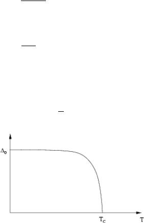
Figure 3.6: Pairing gap as function of temperature

It is important to note, that this is a single particle spectrum, i.e. no collective modes are considered. So if an external field, which acts only on single particles, acts with an amplitude less than no excitations occur. The question remains whether other types of excitations with amplitude less than are possible.

The GOLDSTONE theorem (page 33) ensures that at least one branch of gapless excitations exists because the continuous (gauge) symmetry is spontaneously broken in a superfluid phase: the energy (H AMILTONian) is invariant under the gauge transformation y ! eif y with a constant f, E(eif y) = E(y), while the ground state and, as a result, anomalous correlators are not. For example,

h(eif y)(eif y)i = e2if hyyi 6= hyyi 6= 0:

(3.318)

3.5. BARDEEN-COOPER-SHIEFFER-THEORY	83
Since we have
p!0	(3.319)
ep ! 0

the choice of a phase breaks the symmetry. So if we consider now a phase which varies slowly in space and time, i.e. the gap is of the form

D0 ! D0e2if(~r;t)

(3.320)

we describe collective modes. To calculate D we have to redo the previous calculation except for the fact that D is no longer real. The HAMILTONian is now

		2
Hˆ = åj	Z	d3r yˆ j	~	Ñ2 +U (~r) m	yj
			2m

Z

	d3r	n			†	†	o
				+	+
Here the first addend will be called		ˆ
		H0.

Once more we use a time dependent BOGOLYUBOV-DE GENNES equation (i.e. a canonical transformation):

yˆ		n	n		+ sign( j)v		o
	j	å	n	n j	j	n	j

The calculation is similar to the BOSE case and it is therefore not repeated here. It can be found in the literature. The results are

i~		¶un		ˆ	m)un + Dvn
		¶t		= (H0
i	~	¶vn		= (Hˆ			m)v	n	+ D u	n
		¶t			0

We assume that the phase is switched on adiabaticly, i.e.

D t!∞ D

(~r;t) ! 0

This way, the solutions take the form

un (~r;t ! ¥) = u0n e ient vn (~r;t ! ¥) = v0n e ient

Using this (3.323) and (3.324) read

(0)	ˆ	(0)	(0)
en un	= (H0	m)un	+ D0vn
(0)	ˆ	(0)	(0)
en vn	= (H0	m)vn	+ D0un

(3.323)

(3.324)

(3.325)

(3.326)

(3.327)

(3.328)

(3.329)

84				CHAPTER 3. FERMIONS
Thus n is clear at t = ¥. Now we have to solve self-consistently
D(~r;t) = jV0jhy (~r;t)y+(~r;t)i						(3.330)
		ˆ	ˆ
j	j				en
		n			2T
= V0		åun (~r;t)un (~r;t)tanh				(3.331)

where we took only the leading term in the fluctuations. The probability current at T = 0 reads now

i~

åj

†

†

~

hyj Ñyj Ñyj

yji

j

= 2m

ˆ

ˆ

ˆ

ˆ

=

i~

å å

(v

Ñv

Ñv

v

) a˜

a˜ †

2m

n1

n2

n1

n2 h

n1 j n2 ji

j n1n2

|

n{z1n

}

i~

n

n

n n

d

2

2m

åå

=

j

n

(v

Ñv

Ñv v )

The same way we calculate

n = ååjvn j2

j n

If we define new functions

(3.332)

(3.333)

(3.334)

(3.335)

u	n	= eif u¯	v	n	= e if v¯	(3.336)
		n			n

which obey the same initial conditions (because f vanishes at t = ¥) (3.323) and (3.324) simplify

i~¶t ~f˙ u¯n =

2

(3.337)

2~m (Ñ + iÑf)2 m u¯n + D0v¯n

¶

i~¶t + ~f˙ v¯n =

2

m v¯n + D0u¯n

(3.338)

2~m (Ñ iÑf)2

¶

We have now

i~ ¶t =

2

2~m Ñ2 m u¯n + D0v¯n

¶u¯

+ ~f˙ +

2

~2

~2

Ñ2f u¯n

~

(Ñf)2

i

ÑfÑ

i

(3.339)

2m

m

2m

2

i~¶t = 2~m Ñ2 m v¯n + D0u¯n

¶v¯

+ ~f˙

~2

~2

~2

Ñ2f v¯n

(Ñf)2 i

ÑfÑ i

(3.340)

2m

m

2m

3.5. BARDEEN-COOPER-SHIEFFER-THEORY

85

If we regard f:::g as perturbation we can apply time dependent perturbation theory here. We We will not present detailed calculations here, rather make some comments.

When on the basis of the BOGOLYUBOV-DE GENNES equations (...) we consider single-particle excitations, we restrict ourself only to solutions with positive eigenvalues en > 0. But those are only half of all possible solutions. The other half contains solutions with negative eigenvalues en < 0. The latter can easily be constructed from the former. Namely, if (u(n0);v(n0)) is a solution with en > 0, then, as can be easily checked, (v(n0) ; u(n0) ) is a solution with the negative eigenvalue en < 0. Together they form a complete set of solutions and, therefore, they both have to be used in studying the perturbed BOGOLYUBOV-DE GENNES equations. In this way we get the answer

u¯n = un(0)e ient (1 + derivatives of f)

(3.341)

v¯

= v(0)e ient (1 + derivatives of f)

(3.342)

n

n

After some calculations the current can be written as

j =

2m ån

2iÑfjvn

j + O

D0

;

˙

(3.343)

D0

~

i~

(0)

2

Ñf

f

~

(0) 2

~

=

Ñf åjvn j

= n0

Ñf

= n0~vs

(3.344)

m

m

n

vs =

~

Ñf

(3.345)

m

This result is rather unexpected. It is not obvious that the constant n0 from the homogeneous case is the coefficient and not e.g. a fraction of n0. As can be

Figure 3.7: Schematic probability flow in BCS

seen in figure (3.7) most particles inside the F ERMI sphere are not affected by the probability flow.

86	CHAPTER 3. FERMIONS

Now n and ~vs have to be solved self-consistently to get an equation for f. Here we want to get the solution more easily:

E(f;n) = Z d3r	1	mn~vs2 + E(n) mn
	2

E(n) = Eon(n) + Eint + Ecooper p.

3

= n 5 eF + O(a) + Ecooper p.

| {z }

e l2

(3.346)

(3.347)

(3.348)

Here E0n describes free particles in the normal phase. We can estimate the pairing energy as energy gain per pair times number of particles affected, i.e.

2

mp

F

2

m p3

Ecooper p. ( )n(eF) g

= g

F

(3.349)

~3

pF2

~3

2

neF

2

(3.350)

n

eF

eF

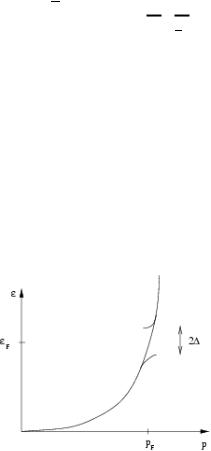
Figure 3.8: BCS gap

Again we note that we consider only slowly varying phase.

If we look at (3.346) with terms up to second order in phase and dn, remembering

n0 :	¶E	= m	(3.351)
	¶n

3.5. BARDEEN-COOPER-SHIEFFER-THEORY

87

we get

d3r

1

~

2

E

n

mn

E

n

linear

0 m Ñf

(f;

) = Z

n

2

+

0( 0) +

=0

+

1 ¶2E

n0

2

| {z }

(3.352)

2 ¶n2

(dn) o

3

~

2

2

¶

2

E

2

= E0(n0)V +

1

n0 dn

(3.353)

2 Z

d

r (n0 m

(Ñf) +

¶n2

)

Here we remember that v Ñf and therefore v2s already second order so we can

use n = n0.

If we look at this from a quantum mechanical point of view, dn becomes an operator. It has to obey

f(~r);dn(~r 0) = id ~r ~r 0

(3.354)

and all other commutators have to vanish.

We have

i

ˆ

1 i

~2

2

dn˙ =

~

~

(3.355)

~

2

~

E;dn =

n0 m ( 2Ñ f)( i)

= n0

Ñ2f = Ñ n0

Ñf = Ñ~j

(3.356)

m

m

that corresponds to the continuity equation. On the other hand

i

1 i ¶2E

1 ¶2E

f˙ =

Eˆ ;f =

2dni =

dn;

(3.357)

~

2

~

¶n2

~

¶n2

therefore,

~

2 ˙

n0

¶2E

2

dn¨ = n0 m Ñ f

= m ¶n2

Ñ

dn

and

(3.358)

¨

n0 ¶2E

2

f =

Ñ

f:

(3.359)

m

¶n2

Eqn. (3.358) and (3.359) are wave equations with the wave velocity

c2 =

n0

¶2E

(3.360)

m ¶n2

88																									CHAPTER 3. FERMIONS
Using (3.5) and (3.6) we can calculate the velocity																									1
c		= m ¶n02					0n0 5 2m											g			n0								(3.361)
		n0 ¶2									3 1 6p2~3														2
	2																								3
							@			2			3		2				2						A
		= m 2m 5													3														(3.362)
											g	~				¶n02 n03
		n0 1 3								6p						¶					5
															2
		n0 1 3 6p2										~3				5 2 1									1 pF2				vF2
															3
		=																					=					=
			m 2m 5								g					3 3 n03									3		m2		3
																					1								(3.363)
			vF
c = p																													(3.364)
				3

This is caused by density fluctuations and differs from zero sound, it is the same as the hydrodynamic sound (BOGOLYUBOV-ANDERSON sound). If the fluctuations couple to density, this GOLDSTONE mode can be excited even if the excitation is less than .

3.6Andreev reflection

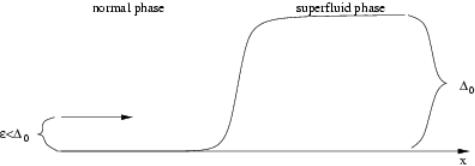
Figure 3.9: Boundary between non superfluid and superfluid region

Suppose we have a situation where the gap is not a constant 0 but depends on the coordinate x in such a way that it is zero for negative x (normal phase), then it increases to its equilibrium value 0 in the transition region of the width x at the origin x = 0, and is equal to 0 for positive x (superfluid phase), see fig.(3.9) (this situation could be realized if a magnetic field is applied to the part x < 0 of the superfluid sample that destroys the C OOPER pairing,).

3.6. ANDREEV REFLECTION

89

If we now have a particle in the normal part of the sample with the energy eF + e, where e < D0, and momentum p > pF along the x-axis (a single-particle excitation with the energy e and momentum p), we would naively expect that it reflects back from the boundary between normal and superfluid parts of the sample because there are no available single-particle states with such energy e < D0 in the superfluid region. However, this is not possible because the change of the momentum d p of the particle in the transition region can be estimated as

d p Ft			F				D0		t =	x	(3.365)
							x			vF
D0			pF	D0		pF					(3.366)
	vF			eF
but an ordinary reflection requires
	Dpjreflection						2pF:				(3.367)

So the particle (excitation) cannot be reflected in a normal way and it cannot penetrate either. What happens instead is that the particle picks another one with an (almost) opposite momentum p0 < pF to form a COOPER pair with total momentum p p0 along the x-axis, and this pair penetrates the superfluid region x > 0. As a result, in the normal region x < 0 one has a hole in the state with momentum p0 moving backwards with the velocity which is a gradient of the energy of the excitation ep0 vF(pF p0) with the respect to its momentum ~p 0 (the hole in the state ~p 0 has momentum -~p 0).

ˆ 0	= vF~ex:	(3.368)
~vout = Ñ p0ep0 Ñp0(vF(pF p0)) vF~p

(For incoming particle one has vin Ñp(vF(p pF)) vF ~ex) Therefore, we have a specific form of a reflection (A NDREEV reflection) where an incoming particle reflects as a hole and vice versa. Since the hole has an opposite charge, some interesting effects happen if a magnetic field is applied - the hole travels the path backwards until it hits the boundary again where it becomes a particle that travels the same path forward and so on.