Dressel.Gruner.Electrodynamics of Solids.2003

88	4 The medium: correlation and response functions
before we start from Heisenberg’s equation (4.3.3) with the interaction term
	HintT =	e
			p(r) · A(r, t) ,	(4.3.24)
		mc

where we have assumed Coulomb gauge · A = 0. Using Bloch states, we can write

ih	∂		k + q, l |δ N |kl = k + q, l |[H0, δ N ]|kl
	∂
¯		t

+k + q, l |[(e/mc) p · A(r, t), N0]|kl

=(Ek+q,l − Ekl ) k + q, l |δ N |kl

+[ f 0(Ekl ) − f 0(Ek+q,l )]

		e
	× k + q, l | mc
			p · A(q , t) exp{i(q · r )} |kl .
			q
			(4.3.25)

With the explicit form of the Bloch wavefunctions from before, the matrix element of the second term becomes

k + q, l |	e		p · A(q , t) exp{i(q · r)} |kl = −1		exp{i(q − q) · Rn }
	mc	q		q
					n
		×	dr p · A(q, t) uk+q,l ukl exp{i(q − q) · r } .			(4.3.26)

We again exploit the periodicity of the lattice (r = Rn + r ) and use expression (4.3.10). Then it is sufficient to examine the sum over states within one unit cell

		e			e
	k+q, l | mc			p·A(q , t) exp{i(q ·r)}|kl = k+q, l | mc p·A(q, t) exp{iq·r}|kl .
			q

(4.3.27) As before we describe the adiabatic switch-on by the factor exp{ηt}, and the left hand side of Eq. (4.3.25) becomes

ih

∂

k + q, l |δ N |kl = (hω − ihη) k + q, l |δ N |kl ,

∂

¯

t

¯

¯

and thus we finally obtain with η → 0

k

+

q, l

|

δ N

kl

=

lim

f 0(Ekl ) − f 0(Ek+q,l )

|

η→0

k

+

q,l

− E

kl

−

hω

−

ihη

E

¯

¯

× k + q, l |

e

p ·

A(q, t) exp{iq · r} |kl . (4.3.28)

mc

In analogy to Eq. (4.3.15), we have now related the induced density matrix δ N to the perturbation applied.

4.3 Response function formalism and conductivity

89

Our aim is to evaluate the conductivity or dielectric constant as a function of frequency and wavevector. Starting from the velocity operator of an electron in an electromagnetic field

v =

eA

+

p

,

mc

m

in first order of A we can write for the current density operator

− Tr exp{−iq · r}

e2

e

J(q) =

N0A(q) − Tr exp{−iq · r}

δ N p

mc

m

−e2

Tr

N

A(q)

e

Tr

exp

iq

r

δ N p

.

(4.3.29)

=

mc

{

} − m

{

{−

·

}

0

}

From comparison with Eq. (4.1.6) the term containing A(q) is the diamagnetic current and is given as

e2 N0
Jd(q) = − mc	A(q) ,	(4.3.30)

where N0 is the total electron density. The second term in Eq. (4.3.29) is known as the paramagnetic current; it can be evaluated by taking |k , l = |k + q, l and by substituting the Bloch wavefunctions. Following the procedure as in Eqs (4.3.16)– (4.3.19) finally leads to

e2 N0

1

e2

J(q) = −

A(q) +

A(q)

mc

m2c

l,l

f 0( kl )

f 0( k q,l )

2

E +

E

− E − ¯

−

¯

k

q, l p kl

. (4.3.31)

×

ω

η

+

| |

k

k q,l

kl

h

ih

Applying Ohm’s law we immediately obtain the transverse conductivity and dielectric constant

σˆ

(q, ω) = i

N0e2

ωm

e2

f 0(

f 0

i

k

q,l )

−

(

kl )

2

lim

E +

E

k

q, l p kl

,

→

l,l

E +

− E − ¯

− ¯

+ η 0 ωm2

k

k q,l

kl

hω ihη

+

| |

(4.3.32)

ˆ(q, ω) = 1 + 4π iσˆ (q, ω)

ω

1

4π N0e2

−

lim

4π

e2

l,l

f 0(Ek+q,l ) − f 0(Ekl )

= −

ω2m

→

0

ω2m2

E +

q,l

− E

kl

− ¯

−

¯

η

k

k

hω

ihη

×

k + q, l |p|kl

2

,

(4.3.33)

90 4 The medium: correlation and response functions

an expression similar to the Lindhard equation for the longitudinal response. There are several differences between these two expressions. First we find an additional contribution (the second term on the right hand side), the so-called diamagnetic current. In the interaction Hamiltonian it shows up as a second order term in A and thus is often neglected. Second the matrix element contains the momentum p = −ih¯ instead of the dipole matrix element. Because of this difference, the pre-factor to the summation in Eq. (4.3.20) is proportional to 1/q2, whereas in Eq. (4.3.33) a 1/ω2 factor appears.

Using a similar procedure to before, we can write down the expression for the real and imaginary parts; however, due to the fact that we have to take the limit and finally the integral over k, this procedure is correct only for the imaginary part:

2(q, ω)

4π 2 e2

f 0( kl ) δ

kl

k q,l

hω

=

ω2m2

l,l

E

$

E − E −

− ¯

%

k

− h¯ ω% k + q, l |p|kl 2 .

− δ $Ek+q,l − Ekl

(4.3.34a)

The real part can then be obtained from (q, ω) as given above by applying the

Kramers–Kronig relation, and we find:

4π N0e2

4π e2

1

f 0(

kl )

1(q, ω) = 1 −

−

k

l,l

kl

k

E

h2ω2

ω2m

m2

E

kl

− E

k−q,l (

E

q,l )2

−

+

− E −

− ¯

k+q,l

kl ( k q,l

kl )2

h2

ω2

| |

1

f 0(Ekl )

k

q, l p

kl

2.

(4.3.34b)

E

− E E +

− E

− ¯

A general expression of the response function, valid when both scalar and vector potentials are present, can be found in [Adl62].

Here the transition matrix element is different from the matrix element which enters into the expression of the longitudinal response Eq. (4.3.12), and is given, for Bloch functions by

+

|

|

= −

ih

+

k

q, l

p

k, l

¯

uk

q,l

uk,l dr .

(4.3.35)

After these preliminaries, we are ready to describe the electrodynamic response of metals and semiconductors, together with the response of various ground states which arise as the consequence of electron–electron and electron–phonon interactions. Of course, this can be done using the current–current (or charge–charge) correlation functions, or using the response function formalism as outlined above, and in certain cases transition rate arguments. Which route one follows is a matter of choice. All the methods discussed here will be utilized in the subsequent chapters, and to a large extent the choice is determined by the usual procedures and conventions adopted in the literature.

Further reading

91

References

[Adl62] S.L. Adler, Phys. Rev. 126, 413 (1962)

[Ehr59] H. Ehrenreich and M.H. Cohen, Phys. Rev. 115, 786 (1959)

[Hau94] H. Haug and S.W. Koch, Quantum Theory of the Optical and Electronic Properties of Semiconductors, 3rd edition (World Scientific, Singapore, 1994)

[Kit63] C. Kittel, Quantum Theory of Solids (John Wiley & Sons, New York, 1963) [Lin54] J. Lindhard, Dan. Mat. Fys. Medd. 28, no. 8 (1954)

[Mah90] G.D. Mahan, Many-Particle Physics, 2nd edition (Plenum Press, New York, 1990)

[Noz64] P. Nozieres,` The Theory of Interacting Fermi Systems (Benjamin, New York, 1964)

[Pin63] D. Pines, Elementary Excitations in Solids (Addison-Wesley, Reading, MA, 1963)

[Pin66] D. Pines and P. Nozieres,` The Theory of Quantum Liquids, Vol. 1 (Addison-Wesley, Reading, MA, 1966)

[Sch83] J.R. Schrieffer, Theory of Superconductivity, 3rd edition (Benjamin, New York, 1983)

Further reading

[Ehr66] H. Ehrenreich, Electromagnetic Transport in Solids: Optical Properties and Plasma Effects, in: The Optical Properties of Solids, edited by J. Tauc, Proceedings of the International School of Physics ‘Enrico Fermi’ 34 (Academic Press, New York, 1966)

[Hak76] H. Haken, Quantum Field Theory of Solids (North-Holland, Amsterdam, 1976)

[Jon73] W. Jones and N.H. March, Theoretical Solid State Physics (John Wiley & Sons, New York, 1973)

[Kub57] R. Kubo, J. Phys. Soc. Japan 12, 570 (1957); Lectures in Theoretical Physics, Vol. 1 (John Wiley & Sons, New York, 1959)

[Pla73] P.M. Platzman and P.A. Wolff, Waves and Interactions in Solid State Plasmas

(Academic Press, New York, 1973)

[Wal86] R.F. Wallis and M. Balkanski, Many-Body Aspects of Solid State Spectroscopy

(North-Holland, Amsterdam, 1986)

5

Metals

In this chapter we apply the formalisms developed in the previous chapter to the electrodynamics of metals, i.e. materials with a partially filled electron band. Optical transitions between electron states in the partially filled band – the so-called intraband transitions – together with transitions between different bands – the interband transitions – are responsible for the electrodynamics. Here the focus will be on intraband excitations, and interband transitions will be dealt with in the next chapter. We first describe the frequency dependent optical properties of the phenomenological Drude–Sommerfeld model. Next we derive the Boltzmann equation, which along with the Kubo formula will be used in the zero wavevector limit to derive the Drude response of metals. The response to small q values (i.e. for wavevectors q kF, the Fermi wavevector) is discussed within the framework of the Boltzmann theory, both in the ω qvF (homogeneous) limit and ω qvF (static or quasi-static) limit; here vF is the Fermi velocity. The treatment of the non-local conductivity due to Chambers is also valid in this limit and consequently will be discussed here. An example where the non-local response is important is the so-called anomalous skin effect; this will be discussed using heuristic arguments, and the full discussion is in Appendix E.1. The response for arbitrary q values is described using the selfconsistent field approximation developed in Section 4.3, where we derived expressions for σˆ (q, ω), the wavevector and frequency dependent complex conductivity for metals.

The longitudinal response is presented along similar lines. The Thomas–Fermi approximation leads to the static response in the small q limit, but the same expressions are also recovered using the Boltzmann equation. The Lindhard formalism is employed extensively to evaluate the dielectric response function χˆ (q, ω) and alsoˆ(q, ω) and σˆ (q, ω), the various expressions bringing forth the different important aspects of the electrodynamics of the metallic state.

For sake of simplicity, we again assume cubic symmetry, and avoid complications which arise from the tensor character of the conductivity.

92

5.1 The Drude and the Sommerfeld models

93

5.1The Drude and the Sommerfeld models

5.1.1The relaxation time approximation

The model due to Drude regards metals as a classical gas of electrons executing a diffusive motion. The central assumption of the model is the existence of an average relaxation time τ which governs the relaxation of the system to equilibrium, i.e. the state with zero average momentum p = 0, after an external field E is removed. The rate equation is

d p	= −	p	.	(5.1.1)
dt
		τ

In the presence of an external electric field E, the equation of motion becomes

	d	p	= −	p	−	eE .
	dt			τ

The current density is given by J = −N ep/m, with N the density of charge carriers; m is the carrier mass, and −e is the electronic charge. For dc fields, the condition d p /dt = 0 leads to a dc conductivity

σdc =	J	=	N e2τ		(5.1.2)
				.
	E		m

Upon the application of an ac field of the form E(t) = E0 exp{−iωt}, the solution of the equation of motion

d2r

m dr

= −eE(t)

(5.1.3)

m

+

dt2

τ dt

gives a complex, frequency dependent conductivity

σ (ω)

=

N e2

τ

1

=

σ

(ω)

+

iσ

(ω)

=

N e2

τ

1 + iωτ

. (5.1.4)

ωτ

ˆ

m

1

1

2

m

1

+

ω2

τ 2

− i

There is an average distance traveled by the electrons between collisions, called the mean free path . Within the framework of the Drude model, = v thτ , wherev th is the average thermal velocity of classical particles, and the kinetic energy

12 m v2 th = 32 kBT at temperature T .

The picture is fundamentally different for electrons obeying quantum statistics, and the consequences of this have been developed by Sommerfeld. Within the framework of this model, the concept of the Fermi surface plays a central role. In the absence of an electric field, the Fermi sphere is centered around zero momentum, and p = h¯ k = 0, as shown in Fig. 5.1. The Fermi sphere is displaced in the presence of an applied field E, with the magnitude of the displacement given by −eEτ /h¯ ; electrons are added to the region A and removed from region B. The equation of motion for the average momentum is the same as given above. Again

94 5 Metals

− eEτ

h

B A

Fig. 5.1. Displaced Fermi sphere in the presence of an applied electric field E. Electrons are removed from region B by the momentum p = −eEτ , and electrons are added in region A. The figure applies to a metal with a spherical Fermi surface of radius kF – or a circular Fermi surface in two dimensions.

with J = −N eh¯ k /m and wavevector k = p/h¯ expression (5.1.4) is recovered. However, the scattering processes which establish the equilibrium in the presence of the electric field involve only electrons near to the Fermi surface; states deep within the Fermi sea are not influenced by the electric field. Consequently the expression for the mean free path is = vFτ , with vF the Fermi velocity, and differs dramatically from the mean free path given by the original Drude model. The difference has important consequences for the temperature dependences, and also for non-linear response to large electric fields, a subject beyond the scope of this book. The underlying interaction with the lattice, together with electron–electron and electron–phonon interactions, also are of importance and lead to corrections to the above description. Broadly speaking these effects can be summarized assuming an effective mass which is different from the free-electron mass [Pin66] and also frequency dependent; this issue will be dealt with later in Section 12.2.2.

The sum rules which have been derived in Section 3.2 are of course obeyed, and

can be easily proven by direct integration. The

f sum rule (3.2.28) for example

follows as

∞

N e2

∞

τ dω

∞ ωp2

d(ωτ )

0

σ1(ω) dω =

0

= 0

m

1 + ω2τ 2

4π 1 + (ωτ )2

ωp2

∞

ωp2 π

ωp2

=

arctan{ωτ }

=

=

,

4π

4π 2

8

0

where we have defined

ωp =

4

π N e2

1/2

.

(5.1.5)

m

5.1 The Drude and the Sommerfeld models

95

This is called the plasma frequency, and its significance will be discussed in subsequent sections.

Before embarking on the discussion of the properties of the Drude model, let us first discuss the response in the limit when the relaxation time τ → 0. In this limit

	π		N e2				N e2
σ1(ω) =				δ{ω = 0}	and	σ2(ω) =		.
	2		m				mω

Here σ2(ω) reflects the inertial response, and this component does not lead to absorption but only to a phase lag. σ1(ω) is zero everywhere except at ω = 0; a degenerate collisionless free gas of electrons cannot absorb photons at finite frequencies. This can be proven directly by showing that the Hamiltonian H which describes the electron gas commutes with the momentum operator, and thus p has no time dependence. This is valid even when electron–electron interactions are present, as such interactions do not change the total momentum of the electron system.

5.1.2 Optical properties of the Drude model

Using the optical conductivity, as obtained by the Drude–Sommerfeld model, the various optical parameters can be evaluated in a straightforward manner. The dc limit of the conductivity is

σ1(ω = 0) = σdc =

N e2τ

=

1

ωp2τ

;

(5.1.6)

m

4π

its frequency dependence can be written as

σˆ (ω) =

σdc

=

N e2

1

=

ωp2

1

(5.1.7)

1 − iωτ

m

1/τ − iω

4π

1/τ − iω

with the components

ωp2τ

1

and

ωp2τ

ωτ

(5.1.8)

σ1(ω) =

σ2(ω) =

.

4π

1 + ω2τ 2

4π

1 + ω2τ 2

Thus, within the framework of the Drude model the complex conductivity and consequently all the various optical parameters are fully characterized by two frequencies: the plasma frequency ωp and the relaxation rate 1/τ ; in general 1/τ ωp. These lead to three regimes with distinctively different frequency dependences of the various quantities.

Using the general relation (2.2.12), the frequency dependence of the dielectric constant is

ω2

ˆ(ω) = 1(ω) + i 2 = 1 − 2 p (5.1.9)

ω − iω/τ

96

5 Metals

Conductivity σ (Ω −1 cm−1)

σ (104 Ω −1 cm−1)

105																												σ1																														(a)
					γ = 16.8 cm−1																							σ2																												νp
104
103				νp = 104 cm−1
																																							γ
102
101
100
10−1
10																																							γ
																												σ1																														(b)
8
6
4																												σ2
2
0
					10−4												10−2							100											102													104
																				Frequency ν (cm−1)

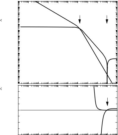
Fig. 5.2. Frequency dependent conductivity σˆ (ω) calculated after the Drude model (5.1.7) for the plasma frequency ωp/(2π c) = νp = 104 cm−1 and the scattering rate 1/(2π cτ ) = γ = 16.8 cm−1 in (a) a logarithmic and (b) a linear conductivity scale. Well below the scattering rate γ , the real part of the conductivity σ1 is frequency independent with a dc

value σdc = 105 −1 cm−1, above γ it falls off with ω−2. The imaginary part σ2(ω)

peaks at γ where σ1 = σ2 = σdc/2; for low frequencies σ2(ω) ω, for high frequencies

σ2(ω) ω−1.

with the real and imaginary parts

		ωp2			1 ωp2
1(ω) = 1	−		and	2(ω) =				. (5.1.10)
		ω2 + τ −2			ωτ		ω2 + τ −2

The components of the complex conductivity σˆ (ω) as a function of frequency

5.1 The Drude and the Sommerfeld models

97

	1010
	10	8				ε2		γ	νp
ε	106					− ε1
constant
	104		γ = 16.8 cm−1
			ν		= 104 cm−1
Dielectric	102			p
	100								ε1
	10− 2
			(a)
	10− 4
ε	20								νp
constant	10							ε2
	0
Dielectric
	−10		(b)						ε1
	−20
			10− 4			10− 2	100	102	104
						Frequency ν (cm−1)

Fig. 5.3. Dielectric constant ˆ(ω) of the Drude model (5.1.9) plotted as a function of frequency in (a) a logarithmic and (b) a linear scale for νp = 104 cm−1 and γ = 16.8 cm−1. For frequencies up to the scattering rate γ , the real part of the dielectric constant 1(ω) is negative and independent of frequency; for ν > γ it increases with ω−2 and finally changes sign at the plasma frequency νp before 1 approaches 1. The imaginary part 2(ω) stays

always positive, decreases monotonically with increasing frequencies, but changes slope from 2(ω) ω to ω−3 at ν = γ .

are shown in Fig. 5.2 for the parameters νp = ωp/(2π c) = 104 cm−1 and γ = 1/(2π cτ ) = 16.8 cm−1; these are typical for good metals at low temperatures. The frequency dependence of both components of the complex dielectric constantˆ(ω) is displayed in Fig. 5.3 for the same parameters.