MODELING, SIMULATION AND PERFORMANCE ANALYSIS OF MIMO SYSTEMS WITH MULTICARRIER TIME DELAYS DIVERSITY MODULATION

and

PSISO = PMISO								= PMIMO .			(4.8)
Therefore, the energy transmitted per antenna P' can be given as
P'	=			PSISO			=		PSISO	.	(4.9)
				L
								2
Now, Equation (4.7) is rewritten as
E'	=	P'T '				=		P T '
									SISO s
s					s			2			(4.10)
			Eb
Es'	=				.
		2

A.SIMULATION OF MDDM TRANSMITTER

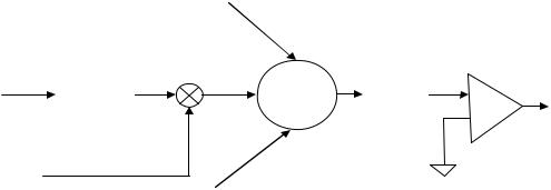
The block diagram of the MDDM transmitter model is shown in Figure 9. The

MDDM transmitter was simulated in MATLAB with equivalent baseband BPSK in the discrete time domain. The simulation was implemented with one sample for each BPSK symbol. The MDDM transmitter scheme, as mentioned in Chapter III with two transmitting antennas, was simulated without added guard interval, D/A converter and RF modulator blocks to facilitate the simulations. Equal power was transmitted from both the antennas. To achieve the same total power transmission as that of a single antenna BPSK transmitter, the signal at each branch of MIMO transmitter was multiplied with a gain factor of g for normalization. The transmitted energy per symbol for BPSK is same

whether a binary 1 or 0 is transmitted. With the gain factor g								the energy per symbol is
represented as
	T '				2
Es' = ∫0 s			gXk				dt = g2A2Ts' .	(4.11)
Substituting Equation (4.10) into Equation (4.11) yields
	P		T '		= g2A2T ' .			(4.12)
	SISO s
2							s

Using Equation (4.2), Equation (4.12) can be rewritten as

51

g2 =		1
		2			(4.13)
g =		1
				.
		2

The gain factor g = 1/ 2 is maintained for all subsequent simulations to transmit the same power as that of a single antenna BPSK system. Thus the effective amplitude of the BPSK modulated signal for each antenna is given as

	Xk		=	A	=	1	.	(4.14)
				2		2

B.SIMULATION OF MDDM RECIVER

The block diagram of the MDDM receiver model is shown in Figure 12. The

MDDM receiver was also simulated in MATLAB with equivalent baseband BPSK in the discrete time domain. The MDDM receiver simulation was implemented as discussed in Chapter III except for the RF demodulator, the A/D converter and the Remove Guard blocks. The receiver was configured as a MISO system with only one receive antenna and as a MIMO system with two receive antennas and as a MIMO system with three receive antennas. After multicarrier delay diversity demodulation, the space diversity receptions of MIMO systems were combined by using the optimum MRC technique as discussed in Chapter II. After the BPSK correlation demodulator as illustrated in Figure 14, ζk (the real part of the random variable Zk ) was compared with the threshold level according to Table 3. For analysis and simulation purposes it is assumed that the transmitter and receiver frequencies are synchronized and, in the case of MIMO systems, all the diversity receptions are also synchronized.

52

l = 1

						Combiner
Rkj					Z kj
		1	T			L
	T ∫0			( )dt		∑	R e [Z k ]	+
						l =1		−

H kj *

l = L

Figure 14 BPSK Correlation Demodulator for MIMO System with MDDM

		Output Binary Bit
ζk	≥ 0	0
ζk	< 0	1

Table 3 Demodulation of BPSK Signal (After Ref. [8]).

C.SIMULATION AND PERFORMANCE ANALYSIS OF MDDM IN AWGN

The performance of MDDM was first simulated and analyzed in AWGN only. In

this simulation and analysis no fading is assumed. This means that each channel response coefficient hlj equals one. A block diagram of the MIMO system in AWGN with three receiving antennas is illustrated in Figure 15. Both the MDDM transmitter and receiver are collapsed into one block each to facilitate presentation. In this simulation two gain blocks each with normalizing gain factor of g are shown at the outputs of the transmitter for each transmitting antenna. The AWGN channel blocks add white Gaussian noise to the signal at respective receiving antennas. The noise power is increased progressively with each simulation run to calculate the bit error rate at different signal to noise ratios. Bit error rate is calculated by comparing the input binary data stream at the input to the

transmitter bk and output binary data stream at the output of the receiver b^k .

53

bk

Tx

^

BER

Calculator

bk

n1

Rx

g

x1

∑

AWGN Channel 1

r1

Gain 1

n2

Random

MDDM

r

2

MDDM

Binary Data

∑

AWGN Channel 2

Tx

Rx

Source

g

x2

r3

Gain 2

n3

∑

AWGN Channel 3

Figure 15 Simulation of MDDM MIMO System in AWGN

1.Performance Analysis of MISO System with Two Transmit and One Receive Antenna

At the receiving antenna, the received signal rm at time m is given by

r	= x1	+ x2	+ n	m	.	(4.15)
m	m	m

where xm2 is a cyclically delayed signal and is given by Equation (3.5)

xm2 = x(1m−1) .	(4.16)
N
After the FFT operation, the received signal is written as

FFT[r	] = FFT[x1	+ x2	+ n	m	].	(4.17)
m	m	m

Using the linearity property of the discrete Fourier transform [13], Equation (4.17) can be represented as

R = X1	+ X2	+ N	.	(4.18)
k k	k	k

Substituting Equation (2.31) and (4.16) into Equation (4.18) yields

R = X		1	+ X1e−j2πk /N	+ N		k
k		k	k				(4.19)
R	= (1	+e−j2πk /N )X1		+ N
					k
k			k

54

where N is	the FFT size or the number of subcarriers, Nk is AWGN in the frequency
domain and	(1 +e−j2πk /N ) is the effective channel response for MDDM in AWGN
channel. To facilitate the presentation, the phase angle φk		is defined as
	φk = 2πk /N.	(4.20)

Multiplying Equation (4.19) by the complex conjugate of the effective channel response, the result is given by

Zk = (1 +e−jφk )(1 +e+jφk )Xk1

+ (1 +e+jφk )Nk .

(4.21)

Using Euler’s identity

ejθ

= cos(θ) + j sin(θ)

(4.22)

Equation (4.21) is rewritten as

Z

k

= (2 + 2 cos(φ ))X1

+ (1 +e+jφk )N

k

.

(4.23)

k

k

Equation (4.23) defines a complex Gaussian random variable Zk

due to AWGN.

For demodulation of BPSK data , ζk

= Re{Zk }

is compared with the threshold as given

in Table 3. If correlation demodulator conditions are assumed then

Tb

A

E{Zk | " 0" was transmitted} = E

1

∫

(2

+ 2 cosφk ) + Nk

(1 +e+jφk ) dt

2

Tb

0

= [2 +

2 cos(φk )]

A

(4.24)

2

= 2 [1 + cos(φk )]A.

Since this expected value is real, it follows that

k

{

{

Z

k }

|"0" was sent

}

=

[

+cos(φ

k

)

]

A

(4.25)

ζ + = E

Re

2 1

The variance of ζk = Re{Zk } is only due to the variance of real part of the noise component (1 +e+jφk )Nk [15, 16] and is represented by σζ2

55

σζ2 = E{(Re (1 +e+jφk )Nk )2}− (E{Re (1 +e+jφk )Nk })2

(4.26)

σζ2 = E{(Re (1 +e+jφk )Nk )2}

where E{ } represents the expected value. ηk = Re (1 +e+jφk )Nk is the real part of a complex Gaussian random variable with zero mean. ηk and ηk2 can be written as

ηk = Re (1 +e+jφk )Nk = 21 ((1 +e+jφk )Nk + (1 +e−jφk )Nk )

ηk2 = (Re (1 +e+jφk )Nk )2 =			1	((1 +e+jφk )Nk + (1		+e−jφk )Nk ) 2
		2						(4.27)
	1	((1 +e+jφk )2 Nk2					+ 2(1 +e−jφk )(1 +e+jφk )NkNk )
=					+ (1 +e−jφk	)2 Nk 2
	4
=	1	((1 +e+jφk )2 Nk2			+ (1 +e−jφk	)2 Nk 2	+ 4(1 + cos(φk ))NkNk ).
	4

where ( ) represents the complex conjugate. Substituting Equation (4.27) into Equation (4.26) gives

σζ2 = E{			1	((1 +e+jφk )2 (Nk )2		+ (1 +e−jφk )2 (Nk )2 + 4(1 + cos(φk ))NkNk )}
			4					(4.28)
=	1	((1 +e+jφk )2 E{(Nk )2}+ (1 +e−jφk )2 E{(Nk )2}+ 4(1 + cos(φk ))E{NkNk }).
	4
As discussed earlier, Nk					is a	complex Gaussian random variable with	zero mean,
therefore
					E{(Nk )2} = E{(Nk )2} = 0 .		(4.29)
Substituting Equation (4.29) into Equation (4.28) gives
					σζ2	= [1 + cos(φk )]E{NkNk }.	(4.30)
Using Equation (2.29), Nk					is given as
						Nk = N∑−1 nme−j2πkm /N .	(4.31)
						m=0

Substituting Equation (4.31) into Equation (4.30) yields

56

		N −1		N −1
σζ2 = [1 + cos(φk )]E ∑nme−j2πkn /N ∑nl e+j2πkl /N
		m=0		l =0
= [1	+ cos(φk )]N∑−1 N∑−1		E{nlnm }e−j2πkl /Ne+j2πkm /N			(4.32)
		l =0 m=0
		N −1 N −1	E n n	e−j2πk(l −m)/N .
= 1	+ cos(φ )	∑∑
[	k ]		{ l m	}

l =0 m=0

Samples of AWGN at different time instants are IID Gaussian random variables with zero mean. Therefore, they are uncorrelated and the variance can be represented as

		E	{nm }E{np }
E{nmnp	}=	E	{		n			2	}
						m
		0
	=		2
		σn		m

if m ≠ p

if m = p

(4.33)

if m ≠ p if m = p.

Substituting Equation (4.33) into Equation (4.32) gives

σζ2 = [1 + cos(φk )]N∑−1	E{nmnm }
m=0	(4.34)
= [1 + cos(φk )]Nσn2m

where σ2 is the noise power of the OFDM symbol in the time domain before the FFT

nm

operation. If correlation demodulator conditions are assumed, the noise power for OFDM symbol durations is given by

	2		No	∞	2
				∫
	σnm	=			H(f )	df	(4.35)
			2
				−∞

where No /2 (Watts per Hertz) is the power spectral density of the real part of noise and

H(f ) is the frequency response of the integrator [15, 16]. Using Parsevel’s theorem [19], Equation (4.35) converts to

57

2

No

Ts

2

∫

σnm

=

h[t]

dt

2

0

No

T

1

=

∫s

dt

2

T 2

0

s

=

No

.

2T

s

Substituting Equation (4.36) into Equation (4.34) gives

σζ2 =

[1 + cos(φk )]NNo

.

2Ts

Substituting, T from Equation (2.33) and since for BPSK T '
s			s
yields
σζ2 =	[1 + cos(φk )]NNo	=	[1 + cos(φk )]No	.
	2NTb
			2Tb

(4.36)

(4.37)

=Tb , Equation (4.37)

(4.38)

Using Equations (4.24) and (4.38), the bit error probability

φk can be expressed as

Pb' = Pr{ζk < 0 | " 0 " was sent}

−

+

+

= Pr ζk

ζk < −

ζk

| " 0 "

σξ

σξ

k

k

−

+

+

= Pr ζk

ζk >

ζk

| " 0 "

σξ

k

σξ

k

Pb' conditioned on the value

(4.39)

						2A(1 + cos(φ ))
		ζ +
=Q		k			=Q	k
	σξk					[1 + cos(φk )]No /2Tb

	=Q	2A Tb [1 + cos(φk )]		=Q	2	Eb [1 + cos(φk )]	.
		No				No

The number of data symbols per OFDM frame is 192 as discussed in Chapter III. The indices of these data symbols are given as k = 9,10,...,100,156,157,...,255 . Thus, the average bit error probability Pb is given by

58

Pb =

1

∑Q

4[1 + cos(φk )]Eb

+ ∑Q

4[1 + cos(φk )]Eb .

(4.40)

100

255

192

No

No

k =9

k =156

The simulation was conducted with increasing

Eb /No for

100,000

OFDM

frames or 19.2 million data symbols per Eb /No

value.

The simulated bit error rate (BER) for the MISO system is plotted in Figure 16

where L = 2

is the number of transmit antennas and J = 1 is the number of receive

antennas. The theoretical probability of bit error as obtained in Equation (4.40) is also plotted. For comparison of performances, this figure also includes the theoretical probability of bit error for a baseband equivalent SISO system. The simulated results follow the theoretical results very closely. The MISO system with MDDM performs better than the SISO system for lower Eb /No values and the performance of the MISO system is poorer than that of SISO system for Eb /No greater than 6.5 dB.

Figure 16 Results of MDDM MISO System in AWGN

59

2.Performance Analysis of MIMO System with Two Transmit and Two Receive Antennas

For the MDDM MIMO system with two receive antennas, it is assumed that the signal receptions at both the antennas are uncorrelated and signals are received at the same time without any relative delay. The received signals at both receive antennas are given by

rm1 = xm1 + xm2 + nm1 rm2 = xm1 + xm2 + nm2 .

After the FFT operation the signals can be represented as

Rk1 = Xk1 + Xk2 + Nk1

Rk2 = Xk1 + Xk2 + Nk2.

Substituting Equation (2.31) and (4.19) into Equation (4.42) gives

R1	= X	1	+ X1e−j2πk /N + N 1
k		k	k	k
R2	= X	1	+ X1e−j2πk /N + N 2
k		k	k	k
R1	= (1	+e−jφk )X1		+ N 1
k			k	k
R2	= (1	+e−jφk )X1		+ N 2.
k			k	k

Following the derivation of Equation (4.23), Equation (4.43) converts to

Zk1 = Rk1(1 +e+jφk ) = [2 + 2 cos(φk )]Xk1 + (1 +e+jφk )Nk1

Zk2 = Rk2(1 +e+jφk ) = [2 + 2 cos(φk )]Xk1 + (1 +e+jφk )Nk2.

Now both space diversity receptions are combined to form random variable Zk given by

Zk = Zk1 + Zk2

= [4 + 4 cos(φk )]Xk1 + (1 +e+jφk )Nk1 + (1 +e+jφk )Nk2

= 4[1 + cos(φk )] A2 + (1 +e+jφk )Nk1 + (1 +e+jφk )Nk2 = 2 2A[1 + cos(φk )]+ (1 +e+jφk )Nk1 + (1 +e+jφk )Nk2.

If correlation demodulator conditions are assumed, then

(4.41)

(4.42)

(4.43)

(4.44)

which is

(4.45)

60