MODELING, SIMULATION AND PERFORMANCE ANALYSIS OF MIMO SYSTEMS WITH MULTICARRIER TIME DELAYS DIVERSITY MODULATION

			1		Tb
E{Zk | " 0" was transmitted} =
	E				∫Zkdt
		T
			b		0
= 2			2A(1 + cos(φk )).				(4.46)
The variance of ζk = Re{Zk } is only due to	the			variance of real part			of noise

components [15, 16]. Noise components at both receive antennas are IID Gaussian random variables. Therefore the total variance of the sum of two noise components is the sum of their individual variances [18]. The total noise variance is given as

			σ 2	= σ 21		+ σ 22				(4.47)
			ζk	ζk			ζk
where	ζk1 = Re{Zk1} and	ζk2	= Re{Zk2 }. Following the derivation							of noise variance
derived in Equation (4.37), Equation (4.47) is represented as
	σζ2	=	[1 + cos(φk )]No		+		[1 + cos(φk )]No
			2Tb				2Tb
	k
			[1 + cos(φk )]No							(4.48)
		=
			Tb
and σζk	is given as
			σζ =	(1 + cos(φk ))No				.		(4.49)
			k			Tb

Following the derivation of Equation (4.39), the bit error probability Pb' conditioned on the value φk is given by

		2 2		[1 + cos(φk )]A
P' =Q
b
		[1 + cos(φk )]No /Tb
		8[1			2
	=Q			+ cos(φk )]A Tb					(4.50)
				No
	=Q	8[1		+ cos(φk )]Eb		.
				No

61

Following the derivation of Equation (4.40) the average probability of bit error MDDM MIMO system with two transmit and two receiving antennas is given by

1

100

8(1 + cos(φ ))E

255

8(1 + cos(φ ))E

b

P =

Q

k

b

+

∑

Q

k

.

b

192

∑

No

No

k =9

k =156

Pb for a

(4.51)

The simulation was conducted for the same number of OFDM frames or data symbols as mentioned in the previous section. The simulated bit error rate (BER) for the MIMO system is plotted in Figure 17. The simulated results follow theoretical results very closely.

1.7 dB

Figure 17 Results of MDDM MIMO System in AWGN

3.Performance Analysis of MIMO System with Two Transmit and Three Receive Antennas

Similarly, in this section, the performance analysis of MDDM MIMO system with two transmit and three receive antennas is discussed. Exploiting the symmetry of the receiver design, the derivation of results is mainly based on the results presented in the

62

last two sections. It is also assumed that the signal receptions at all antennas are uncorrelated and signals are received at the same time without any relative delay. The received signals at the three receive antennas are given by

r1	= x1	+ x2	+ n1
m	m	m	m
r2	= x1	+ x2	+ n2	(4.52)
m	m	m	m
r3	= x1	+ x2	+ n3 .
m	m	m	m

After the FFT operation the signals are represented as

R1	= X1	+ X2	+ N 1
k	k	k	k
R2	= X1	+ X2	+ N 2	(4.53)
k	k	k	k
R3	= X1	+ X2	+ N 3.
k	k	k	k

Based on the discussion in previous sections, the components of the variables from all the space diversity receptions are

Zk1 = Rk1(1 +e+jφk ) = [2 + Zk2 = Rk2(1 +e+jφk ) = [2 + Zk3 = Rk3(1 +e+jφk ) = [2 +

2 cos(φk )]Xk1	+ (1 +e+jφk )Nk1
2 cos(φk )]Xk1	+ (1 +e+jφk )Nk2	(4.54)
2 cos(φk )]Xk1	+ (1 +e+jφk )Nk3.

Now all the space diversity receptions are combined to form random variable Zk which is given by

Zk = Zk1 + Zk2 + Zk3							(4.55)
	= 6[1 + cos(φk )]Xk1 + (1 +ejφk )Nk1			+ (1 +ejφk )Nk2 + (1 +ejφk )Nk3.
If correlation demodulator conditions are assumed, then
			Tb			+jφ
	1
E{Zk	| " 0" was transmitted} = E		∫	2 2A(1	+ cosφk ) + Nk (1 +e	k ) dt
	Tb							(4.56)
			0

= 2	2A[1 + cos(φk )].
The variance of ζk = Re{Zk } is only	due to the variance of real part of noise

components [15, 16]. Noise components at all the receive antennas are IID Gaussian

63

random variables. Therefore the total variance of the sum of three noise components is the sum of their individual variances [18]. The total noise variance is given as

σ 2 = σ 21		+ σ 22	+ σ 2 3
ζk	ζk	ζk	ζk
where ζk1 = Re{Zk1}, ζk2 = Re{Zk2 }	and	ζk2 = Re{Zk2 }. Following the

noise variance derived in Equation (4.37), Equation (4.57) is represented as

	σζ2 =	3[1 + cos(φk )]No
		2Tb
	k
	and σζk is

(4.57)

derivation of

(4.58)

σζ

=

3[1 + cos(φk )]No

.

(4.59)

k

2Tb

Following the derivation of Equation (4.39), the bit error probability P'

conditioned on

b

the value φk

is given by

P'

=Q

3 2 [1 + cos(φk )]A

b

3[1 + cos(φk )]No /2Tb

2

=Q

12[1 + cos(φk )]A Tb

(4.60)

No

=Q

12[1 + cos(φk )]Eb

.

No

The average probability of bit error Pb for this case can be obtained by

Pb =

1

∑Q

12

[1 + cos(φk )]Eb +

∑Q

12[1 + cos(φk )]Eb .

(4.61)

100

255

192

No

No

k =9

k =156

The simulation was conducted for the same number of OFDM frames or data symbols as mentioned in the previous section. The simulated bit error rate (BER) for the MIMO system is plotted in Figure 18. The simulated results follow theoretical results very closely.

64

A comparison of Equations (4.40), (4.51) and (4.61) clearly reveals that the improvement factor increases linearly with increasing number of receiving antenna. Thus, the average probability of bit error in AWGN channel for MDDM scheme discussed in this thesis with J receiving antenna can be represented in general form as

1

100

4J(1 + cos(φ ))E

255

4J(1 + cos(φ ))E

P =

Q

k b

+

∑

Q

k

b

.

(4.62)

b

192

∑

No

No

k =9

k =156

3.4 dB

Figure 18 Results of MDDM MIMO System in AWGN

D.SIMULATION AND PERFORMANCE ANALYSIS OF MDDM IN A MULTIPATH FADING CHANNEL

Next, the MDDM scheme was simulated and analyzed with the effect of a slow

fading frequency nonselective channel. The multipath model for the slow Rayleigh fading channel was discussed in Chapter II. A multipath fading channel is inserted in Figure 15 from each transmit antenna to each receive antenna. A block diagram of the MIMO

65

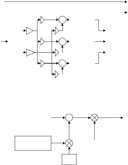
system with slow fading frequency nonselective channel plus AWGN is illustrated in Figure 19. It is assumed that the each channel frequency response remains constant for an OFDM symbol duration. Therefore the channel is slow fading. The simulated channel response is the complex sum of two IID Gaussian random sources. The block model of channel response is illustrated in Figure 20. In simulation, each channel response is multiplied with the transmitted signal from the respective antenna and input to the AWGN block of respective receive antenna.

bk

Tx

^

BER

Calculator

bk

h

11

n1

Rx

∑

AWGN Channel 1

g

x1

h21

r1

Gain 1

h12

n2

Random

MDDM

r

2

MDDM

Binary Data

∑

AWGN Channel 2

Tx

Rx

Source

h22

g

x2

r3

Gain 2

h13

n3

AWGN Channel 3

∑

h23

Figure 19 Simulation of MDDM MIMO System in Multipath

			hlj		ejθ	xl		hlj		ejθ
Gaussian Random	∑
Source 1

	Gaussian Random	xl
	Source 2

j

Figure 20 Simulation of Channel Response

66

FFT[rm ] = FFT[h11xm1 + h21xm2 + nm ].

Each Gaussian random source generates a zero mean random variable. In this simulation model, the variance of each Gaussian source is equal and is set to a value such that the variance of the complex sum of these Gaussian random sources is one. Using Equation (2.52), the channel response from transmit antenna l to receive antenna j is represented as

hlj = hlj ejθlj

(4.63)

= X + jY

where X and Y are IID Gaussian random variables with zero mean and equal variance. The variance of the complex sum can be given as

σh2lj = E {hljhlj*}− (				E {hlj }		)2
{							}
= E (X	+ jY )(X + jY )*
{	+Y 2	}					(4.64)
= E X2

=σX2 + σY2

=1.

Thus the variance of each Gaussian random source was set as

σ2	= σ2	= 1/2.	(4.65)
X	Y

1.Performance Analysis of MISO System with Two Transmit and One Receive Antenna

At the receive antenna, the signal rm is written as

r	= h11x1	+ h21x2	+ n	m	.	(4.66)
m	m	m

where h11 and h21 are channel responses from transmit antenna 1 and 2 to the receive antenna respectively. These channel responses are assumed independent. After the FFT operation, the signal is written as

(4.67) All the channel responses are considered constant for the duration of an OFDM symbol for the slow fading channel. Now, Equation (4.67) can be written as

R = h11X1		+ h21X2	+ N	k	.	(4.68)
k	k	k

67

Substituting Equation (2.31) , (4.16) and (4.20) into Equation (4.68) yields

R = h11X1		+ h21X1e−jφk + N			k
k	k	k				(4.69)
R = (h11	+ h21e−jφk )X1		+ N
				k
k		k

where Nk is AWGN in the frequency domain and (h11 + h21e−jφk ) is the effective channel response for the MDDM in the multipath channel. In Equation (4.69) h21 is a random variable with Rayleigh distributed amplitude and phase uniformly distributed on (−π,π] . Thus, multiplying h21 by e−jφk does not change the statistics of the random variable and their product is represented as h21' . Now, the effective channel response can be written as

H 1 = h11 + h21'

(4.70)

Using the MRC receiver as shown in Figure 14, Equation (4.69) is multiplied by the complex conjugate of the effective channel response and the and random variable Zk is represented as

Zk = H 1H 1*Xk1 + H 1*Nk .

(4.71)

Now, Equation (4.71) can be written as

Zk =

H 1

2 Xk1 + H 1*Nk

= (h11 + h21' )(h11 + h21' )* Xk1 + (h11 + h21' )* Nk

(4.72)

= (

h11

2 +

h21'

2 + 2(hI11hI21' + hQ11hQ21' ))Xk1 + (h11

+ h21' )* Nk

where hlj = hIlj + jhQlj , i.e. hIlj and hQlj are the inphase and quadrature components of the respective channel responses.

For a fixed set of channel responses Equation (4.72) represents a complex Gaussian random variable Zk due to AWGN [16]. To demodulate the BPSK signal, the real part of the decision variable Zk , ζk = Re{Zk }, is compared with a threshold as given in Table 3. If correlation demodulator conditions are assumed, then

68

ζk+ = E{Re{Zk } | " 0 " was transmitted}

1

Tb

11

2

21'

2

11

21'

11

21'

1

11

21'

*

= E

∫

h

+

h

+ 2 (hI hI

+ hQ hQ

)Xk +

(h

+ h

) Nk dt

(4.73)

T

b

0

=

h11

2 +

h21'

2

+ 2 (hI11hI21'

+ hQ11hQ21' )

A

ζk

2

The variance of

is only due to the variance of real part of the noise component

H 1*Nk

[15, 16] and is represented as

σζ2k =

{

H 1*Nk )2

}

− (E{Re H 1*Nk })2

E

(Re

(4.74)

= E{(Re H 1*Nk )2}

where

E{ } represents the expected value. ηk

is the real part of noise component with

zero mean which can be written as

1*

1

1*

1

*

ηk

=

Re

H Nk =

(H Nk

+ H Nk )

(4.75)

2

And

2

1*

2

1

1*

1

*

2

ηk = (Re H Nk

)

=

(H Nk

+

H Nk

)

2

+ 2H 1H 1*NkNk )

=

1

((H 1* )2 Nk2

+ (H 1 )2 (Nk )2

(4.76)

4

=

1

((H 1* )2 Nk2 + (H 1 )2 (Nk )2 + 2

H 1

2 NkNk ).

4

Substituting Equation (4.74) into Equation (4.75) yields

σζ2k = E{

1

((H 1* )2 Nk2 + (H 1 )2 (Nk )2 + 2

H 1

2 NkNk )}

4

(4.77)

=

1

((H 1* )2 E{(Nk )2}+ (H 1 )2 E{(Nk )2}+ 2

H 1

2 E{NkNk }).

4

Nk is a complex Gaussian random variable with zero mean, therefore

E {(Nk )2} = E {(Nk )2} = 0 .

(4.78)

Substituting Equation (4.78) into Equation (4.77) yields

69

2		2					1		2
σζk	=			H								E{NkNk					}
		4
																	(4.79)
	=	1	(			h11					2 +			h21'		2	+ 2(hI11hI21' + hQ11hQ21' ))E{NkNk }.
		2

Now, Equation (4.79) can be written as

σζk

=

1

h

2

+ h

2

+ 2 (hI hI

+ hQ hQ

)

No

2

11

21'

11

21'

11 21'

2

2T

b

11

2

21'

2

11

21'

11 21'

No

σζk

=

h

+

h

+ 2 (hI hI

+ hQ hQ

)

.

4T

b

Now, the conditional bit error probability can be represented as

Pb' = Pr{ζk < 0 | " 0 " was sent}

− ζ

+

ζ

+

= Pr

ζ

k

k

< −

k

| " 0 "

σζ

k

σζ

k

−

ζ

+

ζ

+

= Pr

ζ

k

k

>

k

| " 0 "

σζ

k

σζ

k

ζ +

=Q

k

σ

ζk

(

h11

2

+

h21'

2

+ 2(hI11hI21'

+ hQ11hQ21' ))A/ 2

=Q

2

2

11

+

h

21'

11

21'

11

21'

(

h

+ 2(hI

hI

+ hQ hQ ))No

/ 4Tb

2A2Tb (

h11

2

+

h21'

2

+ 2(hI11hI21'

+ hQ11hQ21' ))

=Q

No

or

2E β

1

Pb'(β1) =Q

b

No

where β1 is given as

β1

=

h11

2

+

h21'

2 + 2

(hI11hI21'

+ hQ11hQ21' ).

(4.80)

(4.81)

(4.82)

(4.83)

Equation (4.82) depicts the bit error probability of a MDDM MISO system conditioned on the random variable β1 . The performance of an MDDM MISO system over a

70