6. Spacetime algebra and Dirac theory

Just as it is possible to describe geometric algebra as a fermionic deformed superanalysis it is also possible to describe spacetime algebra in this context. The basis vectors of space-time are the Grassmann elements γ₀, γ₁, γ₂, and γ₃, which fulfill

(6.1)

where we choose here g_μν = diag(1, −1, −1, −1). The corresponding Clifford star product in space-time is

(6.2)

A general supernumber in space-time has the form

A=a0+a^μγμ+a^μνγμγν+a^μνργμγνγρ+a4I4,

(6.3)

where I₄ = γ₀γ₁γ₂γ₃ and only linearly independent terms should appear. With the four-dimensional pseudoscalar I₄ and the Clifford star product (6.2) it is possible to construct analogously to (3.36) the dual basis γ^μ, which gives γ⁰ = γ₀ and γⁱ = −γ_i. Furthermore one can define in analogy to the three-dimensional case a trace:

(6.4)

The Berezin integral acts here again like a projector on the scalar part of F. The definition of the trace by projecting on the scalar part was already given in [19] and it was also stated that the use of geometric algebra greatly simplifys all the trace calculations usually done in the matrix formalism. An explicit expression for the trace can now in the formalism of deformed superanalysis be given by the Berezin integral.

The question is now how a spacetime vector x=x^μγ_μ is related to its space vector part x=xⁱσ_i. In the γ₀-system this can be seen by a space-time split which amounts to star-multiplying by γ₀:

xCγ0=x·γ0+xγ0=t+x.

(6.5)

One should note that x=xγ₀=x¹γ₁γ₀+x²γ₂γ₀+x³γ₃γ₀ is a spacetime bivector, but on the other hand it is also a space vector because the two-blades γ_iγ₀ behave like σ_i:

(6.6)

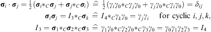
where the four-dimensional star product (6.2) and the three-dimensional star product (3.14) is used in (6.6), as should be clear from the context. The square of the position four vector is x²_C=t²-x²_C.

If a particle is moving in the γ₀-system along x (τ), where τ is the proper time, the proper velocity is given by , with u²_C=1. For the space-time split of the proper velocity one obtains:

(6.7)

Comparing the scalar and the bivector part leads to

(6.8)

and with one gets [3]

(6.9)

It is now also possible to specify a Lorentz transformation from a coordinate system γ_μ to a coordinate system moving in the γ₁-direction. For the coefficients this transformation is given by t = γ (t^′ + βx^′1), x¹ = γ (x^′1 + βt^′), x² = x′², and x³ = x^′3. The condition leads then to

(6.10)

Introducing the angle α so that β = tanh (α) this can be written as

(6.11)

or with as . In general the generators of a passive Lorentz transformation can be calculated with

(6.12)

so that the generators for the boosts and the rotations are

(6.13)

These generators satisfy

(6.14)

and a passive Lorentz transformation is given by

(6.15)

which is a generalization of (6.11).

The Dirac equation can then be written down immediately as [7]

(6.16)

where no slash notation is needed, because one naturally has p=p^μγ_μ. The Wigner function for the Dirac equation is the functional analog of the well-known energy projector of Dirac theory:

(6.17)

Besides the energy one also has the spin as an observable, which is here given by

(6.18)

where s=s^μγ_μ is a vector which fulfills s²_C=-1 and s · p = 0. γ₅ is here γ₅ = iI₄. With and [S_s,pm]_C=0 one sees that the spin Wigner function is given by the functional analog of the spin projector in Dirac theory

(6.19)

and fulfills . The total Wigner function is then the Clifford star product of the two single Wigner functions.