1.4. THE FLAME ALGORITHMIC NOTATION

		PECO	TESLA2
Type of machine		Cluster of SMP	SMP
Number of nodes		4	-
Processor		Intel Xeon E5520	Intel Xeon E5440
Processor codename		Nehalem	Harpertown
Frequency		2.27 Ghz	2.83 Ghz
Number of cores		8	8
Available memory		24 Gbytes DDR2	16 Gbytes DDR2
Interconnection network		Infiniband QDR	-
GPU		NVIDIA Tesla C1060	NVIDIA Tesla S1070
Interconnection bus		PCIExpress 2.0	PCIExpress 2.0
Available memory		4 Gbytes DDR3	16 Gbytes DDR3

Table 1.1: Description of the hardware platforms used in the experiments. The features of PECO are referred to each node of the cluster.

node of PECO. This machine will be the base for the experimental process of the multi-GPU implementations described in Chapter 5.

LONGHORN is a distributed-memory machine composed of 256 nodes based on the Intel Xeon technology. It presents four Intel Xeon 5540 (Nehalem) Quadcore processors per node running at 2.13 Ghz, with 48 Gbytes of DDR2 RAM memory each. Attached to the PCIExpress 2.0 bus of each node, there are two NVIDIA Quadro FX5800 GPUs with 4 Gbytes of DDR3 RAM memory. Nodes are interconnected using a fast QDR Infiniband network. This machine will be the testbed for the experimental stage in Chapter 6.

A more detailed description of the hardware can be found in Tables 1.1 and 1.2. In the selection of those machines, we have chosen those graphics processors and general-purpose processors as close in generational time as possible. This makes it possible to fairly compare single-GPU, multi-GPU and distributed-memory implementations with minimal deviations.

1.3.3.Software description

The software elements used in our work can be divided in two di erent groups. The GPU-related software is selected to be as homogeneous as possible to allow a fair comparison of the di erent platforms. Note that many of the routines presented in the document employ the BLAS implementation (NVIDIA CUBLAS). This implies that experimental results will ultimately depend on the underlying BLAS performance. However, each technique introduced in this research is independent of the specific BLAS implementation. Thus, we expect that when future releases of the NVIDIA CUBLAS library (or other alternative implementations of the BLAS) appear, the performance attained by our codes will be improved in the same degree as the new BLAS implementation. In all the experiments, we employed CUDA 2.3 and CUBLAS 2.3. MKL 10.1 has been used for the CPU executions of the codes in all machines.

1.4.The FLAME algorithmic notation

Many of the algorithms included in this document are expressed using a notation developed by the FLAME (Formal Linear Algebra Methods Environment) project. The main contribution of

13

CHAPTER 1. MATRIX COMPUTATIONS ON SYSTEMS EQUIPPED WITH GPUS

		Per Node		Per System
Type of machine		Cluster of SMP
Number of nodes			256
Processor		Intel Xeon E5440
Processor codename		Nehalem
Frequency		2.53 GHz
Number of cores		8		2,048
Available memory		48 Gbytes		13.5 Tbytes
Interconnection network		Infiniband QDR
Graphics system		128 NVIDIA Quadro Plex S4s
GPU		2 x NVIDIA Quadro FX5800		512 x NVIDIA Quadro FX5800
Interconnection bus		PCI Express 2.0
Available memory		8 Gbytes DDR3		2 Tbytes DDR3
Peak performance (SP)		161.6 GFLOPS		41.40 TFLOPS
Peak performance (DP)		80.8 GFLOPS		20.70 TFLOPS

Table 1.2: Detailed features of the LONGHORN cluster. Peak performance data only consider the raw performance delivered by the CPUs in the cluster, excluding the GPUs.

this project is the creation of a new methodology for the formal derivation of algorithms for linear algebra operations. In addition to this methodology, FLAME o ers a set of programming interfaces (APIs) to easily transform algorithm into code, and a notation to specify linear algebra algorithms. The main advantages of the FLAME notation are its simplicity, concretion and high abstraction level.

Figure 1.2 shows an algorithm using the FLAME notation for the decomposition of a matrix A into the product of two triangular factors, A = LU, with L being unit lower triangular (all diagonal elements equal 1) and U upper triangular. In this case, the elements of the resulting matrices L and U are stored overwriting the elements of A.

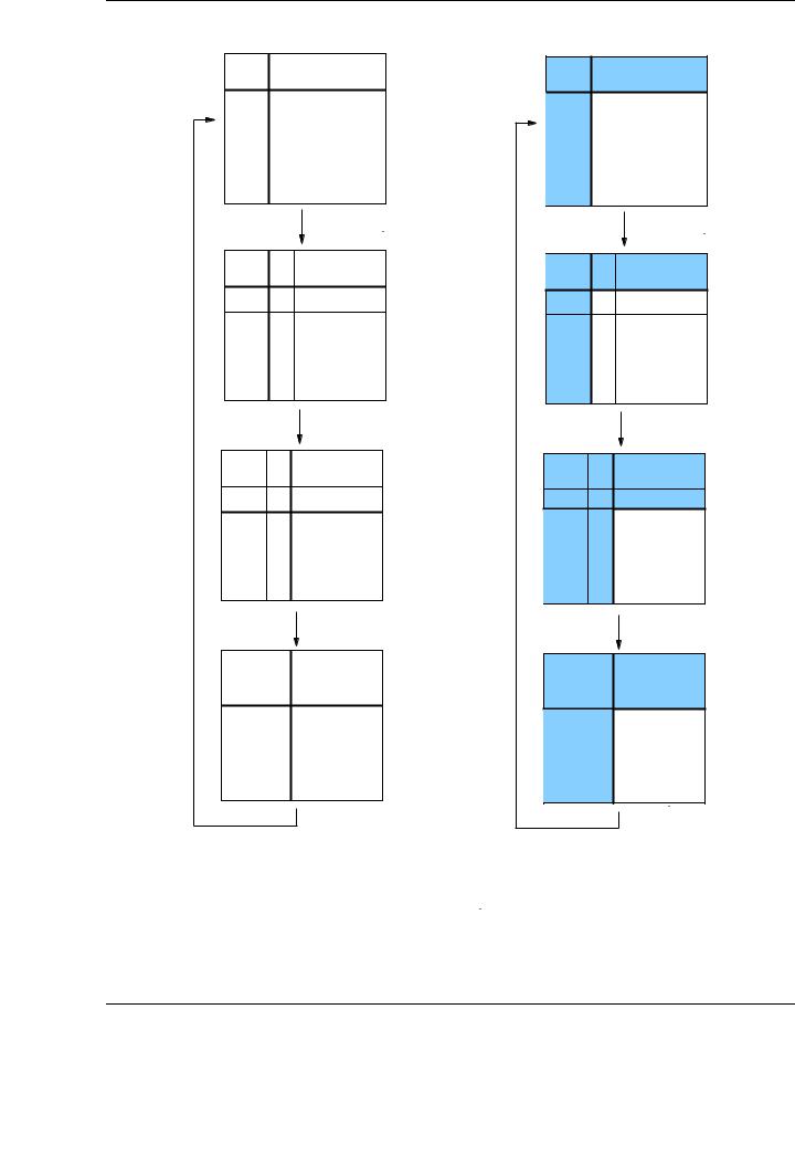
Initially the matrix A is partitioned into four blocks AT L, AT R, ABL, ABR, with the first three blocks being empty. Thus, before the first iteration of the algorithm, the block ABR contains all the elements of the matrix A.

For each iteration, the block ABR is divided, as shown in Figure 1.3, into four blocks: α11, a21, aT12 and A22, and thus being partitioned into 9 blocks). The elements of the L and U factors corresponding to the first three blocks are calculated during the current iteration, while A22 is updated accordingly. At the end of the current iteration, the 2 × 2 partition of the matrix is recovered, and ABR corresponds to the sub-matrix A22. Proceeding in this manner, the operations of the next iteration will be applied again to the recently created block ABR.

The algorithm is completed when the block ABR is empty, that is, when the number of rows of the block AT L equals the number of rows of the whole input matrix A and, therefore, AT L = A. Using the FLAME notation, the loop iterates while m(AT L) < m(A), where m(·) is the number of rows of a matrix (or the number of elements of a column vector). Similarly, n(·) will be used to denote the number of columns in a matrix (or the number of elements in a row vector).

It is quite usual to formulate an algorithm by blocks for a given operation. These algorithms are easily illustrated using the same notation, in which it is only necessary to include an additional parameter: the algorithmic block size. This is a scalar dimension that determines the value of the blocks involved in the algorithms and is usually denoted by the character b.

14

1.4. THE FLAME ALGORITHMIC NOTATION

Algorithm: A := LU(A)

Partition

A →

AT L

AT R

!

ABL

ABR

where AT L is 0 × 0

while

m(AT L) < m(A)

do

Repartition

AT L

AT R

! →

A00

a01

A02

T

T

ABL

ABR

a10

α11

a12

A20

a21

A22

where

α11 is a

scalar

α11

:=

v11 = α11

a12T

:=

v12T = a12T

a21

:=

l21 = a21/v11

A22

:=

A22 − l21 · v12T

Continue with

AT L

AT R

A00

a01

A02

! ←

a10T

α11

a12T

ABL

ABR

A20

a21

A22

endwhile

Figure 1.2: Algorithm for the LU factorizaction without pivoting using the FLAME notation.

15

CHAPTER 1. MATRIX COMPUTATIONS ON SYSTEMS EQUIPPED WITH GPUS

AT L AT R

ABL ABR

A00

α11 aT12

a21 A22

A00

α11 aT12

a21 A22

AT L AT R

ABL ABR

CALCULAT ED

ED		P artially
LAT
		updated
CALCU
		CALCULAT ED
ED
LAT		P artially
		updated
CALCU
		CALCULAT ED
ED
LAT		P artially
CALCU		updated
		CALCULAT ED
	ED	P artially
	LAT
		updated
	CALCU

Figure 1.3: Matrix partitions applied to matrix A during the algorithm of Figure 1.2.

16

1.4. THE FLAME ALGORITHMIC NOTATION

The FLAME notation is useful as it allows the algorithms to be expressed with a high level of abstraction. These algorithms have to be transformed into a routine or implementation, with a higher level of concretion. For example, the algorithm in Figure 1.2 does not specify how the operations inside the loop are implemented. Thus, the operation A21 := A21/v11 could be executed by an invocation to the routine SCAL in BLAS-1; alternatively, this operation could be calculated using a simple loop. Therefore, it is important to distinguish between algorithm and routine. In the following chapters we will show how the FLAME/C API allows an almost straightforward translation of the algorithms into high performance C codes.

17

CHAPTER 1. MATRIX COMPUTATIONS ON SYSTEMS EQUIPPED WITH GPUS

18