10.3 Offender Residence Prediction

As early as 1986, LeBeau recognized the investigative potential of geostatistical techniques and crime pattern research for reducing the offender search area in rape cases. Until the development of geographic profiling in 1990, however, there was no tested systematic method beyond centrography for approaching this problem. Taylor (1977) states that geographic patterns should be viewed through the processes that produce them. Accordingly, crime pattern theory was utilized as a heuristic for the construction of an algorithmic model for locating offender residence (see Benfer et al., 1991). The research of Brantingham and Brantingham interprets offenders’ activity spaces in order to describe where crimes are most likely to occur. Geographic profiling is, in effect, an attempt to invert this model, by using crime locations as the basis for predicting most probable area of offender residence or workplace. So while the two models have different purposes and inputs, their underlying concepts and ideas are similar.

10.3.1 Criminal Geographic Targeting

In the simplest case, offenders’ residences lie at the centre of their crime patterns and can be found through the spatial mean. The intricacy of most criminal activity spaces, however, indicates that more complex patterns are the norm. George Rengert (1996) proposes four hypothetical spatial patterns for the geography of crime sites: (1) uniform pattern, with no distance-decay influence; (2) bull’s-eye pattern, exhibiting distance decay and spatial clustering around the offender’s anchor point; (3) bimodal pattern, with crimes clustered around two anchor points; and (4) teardrop pattern, centred around the offender’s primary anchor point, with a directional bias towards a secondary anchor point. Crime patterns are also distorted by a variety of other real world factors — movement follows street layouts, traffic flows affect mobility, variations exist in zoning and land use, and crimes cluster dependent upon the nature of the target backcloth. The spatial mean is therefore limited in its ability to determine criminal residence.

Many researchers have noted the importance of direction as well as distance in the analysis of spatial patterns of criminal behaviour. Rengert and Wasilchick (1985) found a directional bias towards burglars’ workplace and recreation sites. Canter and Hodge (1997) noticed that while crimes of U.S. and British serial killers generally grouped around their homes, they were also biased towards other activity sites. In their Sheffield study, Baldwin and Bottoms (1976) observed that crime disproportionately occurs in the city centre, indicating offender preference for such a bearing. Nonparametric assessments of spatial autocorrelation in the orientation of criminal travel

© 2000 by CRC Press LLC

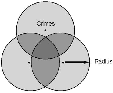
Figure 10.1 Journey-to-crime Venn diagram.

suggests that directional information can assist in certain police investigations (Costanzo, Halperin, & Gale, 1986).

Environmental criminology establishes a framework within which jour- ney-to-crime research, centrography, and other geographic principles may be combined to create a method for determining offender residence from crime locations. Set theory provides a useful first approach for addressing this problem (Taylor, 1977). The ATF/FBI research on serial arsonists found that 70% set fires within 2 miles of their home. Figure 10.1 shows a Venn diagram for three hypothetical serial arsons.63 The medial circles surrounding each crime location are defined by a radius equal to journey-to-crime distance d, within the range of which percentage p of the offender’s arsons occur (d = 2 miles; p ≥ 0.70). The probability of the offender’s residence lying within the area circumscribed by a single circle is therefore also p. Because the crimes are connected, the lune overlap areas between any two circles is more likely to contain the offender’s residence. The highest probability is in the middle region where all three of the circles intersect.

The residence of the offender is most likely within (in decreasing order of probability): (1) the middle intersection; (2) the lunes; (3) the circles; and

(4) the background area. The areal probabilities for the four different spaces

63 This procedure is akin to constructing an intersection of investigative frames through the use of geographic information (Kind, 1987b).

© 2000 by CRC Press LLC

delineated by the Venn diagram in Figure 10.1 are given in Equations 10.1 to 10.4:

p(C ) = p		(1 – p	)2	(10.1)
i	d	d
p(Ci ∩ Cj) = pd2 (1 – pd)				(10.2)
p(Ci ∩ Cj ∩ Ck) = pd3				(10.3)
p((Ci ∩ Cj ∩ Ck)′) = (1 – pd)3				(10.4)

where:

p(A) is the probability the offender’s residence lies within area A;

Cx	is the area around crime site x circumscribed by radius d; and
pd	is the probability the offender’s crime journey is less than or
	equal to d.

Relative probabilities for the points within the various areas are obtained by dividing the areal probabilities by area size (or number of “points”). This process is a simple dichotomous function dependent only upon whether a point lies within one of the circles or not. Points in the overlaps of two, or all three of the circles, are given double or triple the value, respectively.

This process is conceptually similar to the function of the criminal geographic targeting algorithm, the primary tool used in geographic profiling, but dichotomizing distance oversimplifies journey-to-crime patterns. The Brantingham and Brantingham model suggests the criminal search process is more correctly modeled by a distance-decay curve, incorporating a buffer zone centred around the residence of the offender. A more sophisticated method of predicting offender residence location results therefore by replacing the circles in Figure 10.1 with a Pareto function f (d ), in a fuzzy logic approach that better describes journey-to-crime behaviour (Kosko & Isaka, 1993; Yager & Zadeh, 1994): the value assigned to point (x, y), located at distance d from crime site i, equals f (di). The final value for point (x, y) is determined by adding together the n values derived for that point for the n different crime sites.

Research conducted at Simon Fraser University and the Vancouver Police Department following this approach led to the development of the criminal geographic targeting (CGT) model which has been developed into a computerized geographic profiling system. Crime site coordinates are analyzed with a patented criminal hunting algorithm that produces a probability surface showing likelihood of offender residence within the hunting area. A three-dimensional depiction of this probability is referred to as a jeopardy

© 2000 by CRC Press LLC

surface. A two-dimensional perspective integrated with a street map is termed a geoprofile. These are discussed further, and examples shown, below.

The hunting area is defined as the rectangular zone oriented along the street grid containing all crime locations. These locations may be victim encounter points, murder scenes, body dump sites, or some combination thereof. The term hunting area is therefore used broadly in the sense of the geographic region within which the offender chose — after some form of search or hunting process — a series of places for criminal action. Locations unknown to authorities, including those where the offender searched for victims or dump sites but was unsuccessful or chose not to act, are obviously not included.

While the primary purpose of determining offender hunting area is calculation of search area size, there may be other value in such measures. The FBI used convex hull polygons to analyze the point patterns formed by serial rapists (Warren et al., 1995). For local serial rapists (travel under 20 miles), the mean CHP area was 7.14 square miles. The average CHP size was larger for commuters than for marauders (11.38 vs. 7.62 mi2), for rapists who burgled (15.24 vs. 2.49 mi2), and for offenders who lived outside of the CHP area enclosing their crimes (23.53 vs. 3.22 mi2). If replicated, this last finding could be useful in helping narrow offender residence area in cases of serial rape.

Any geometric method of determining hunting area has strengths and weaknesses, and the optimal approach depends ultimately upon the underlying purpose. Many predators exhibit a high hunting to offending ratio. A priori, we do not know where this hunting area is — we only know the locations of the reported, and connected, crimes. Technically, a geoprofile stretches to infinity; the hunting area is only a standardized method of displaying results so that important information is shown, and unimportant information is not. Special methods are used to deal with unusual patterns, including elimination of outliers, division of crimes into separate analyses, and geometric transformations of point patterns (e.g., rotations, “straightening,” trimming, reflections, etc.). The decision on how to proceed is ultimately based on the crime locations and their underlying landscape, guided by theory and methodology. Criminal geographic targeting considers offender hunting methods and mental maps within a framework informed by routine activity, rational choice, and pattern theories.

The CGT analysis uses a Manhattan metric. This may appear to be a less than optimal approach for crimes in cities characterized by concentric, as opposed to grid, street layouts. Model testing and experiences with European cases have demonstrated otherwise. The Manhattan metric slightly overestimates travel in a concentric street layout, but crow-flight distance in turn results in a small underestimate. Neither are far off; on average, the Manhat-

© 2000 by CRC Press LLC

tan distance is approximately 1.273 times the length of the crow-flight distance (Larson & Odoni, 1981). Wheel distance, or path routing, is the most accurate estimate of shortest available travel distance — which may or may not be the actual route taken. It is less the physical distance than its psychological perception that is important. Factors such as traffic congestion, travel time, cost, and familiarity will influence “distance,” regardless of the metric used.

The CGT model follows a four-step process:

1.Map boundaries delineating the offender’s hunting area are first calculated from the crime locations. In the case of a Manhattan grid oriented along northerly and easterly axes, borders are determined by adding edges equal to 1/2 the mean x and y interpoint distances to the most eastern and western, and northern and southern points, respectively (for a discussion of alternative techniques for dealing with edge effects, see Boots & Getis, 1988):

yhigh = ymax + (ymax – ymin)/2 (C – 1)	(10.5)
ylow = ymin – (ymax – ymin)/2 (C – 1)	(10.6)
xhigh = xmax + (xmax– xmin)/2 (C – 1)	(10.7)
xlow = xmin – (xmax – xmin)/2 (C – 1)	(10.8)

where:

yhigh is the y value of the northernmost boundary; ylow is the y value of the southernmost boundary;

ymax is the maximum y value for any crime site; ymin is the minimum y value for any crime site; xhigh is the x value of the easternmost boundary;

xlow is the x value of the westernmost boundary;

xmax is the maximum x value for any crime site; xmin is the minimum x value for any crime site; and

Cis the number of crime sites.

2.For every point on the map, Manhattan distances to each crime location are determined. While there are an infinite number of mathematical points in an area, the model uses a finite number of pixels (40,000) based on the measurement resolution of the x and y scales.

3.The distance is used as an independent variable in a distance decay function; if the distance is less than the radius of the buffer zone,

©2000 by CRC Press LLC

however, the function is reversed. Values are computed for each crime location (e.g., 12 crime locations equates to 12 values for every map point).

4.These values are summed64 to produce a final score for each map point. The higher the resultant score, the greater the probability that point contains the offender’s anchor point. The score function is presented in Equation 10.9:

C

pij = k∑ φ / (

xi − xn

+

yj − yn

)f +

n=1

(10.9)

(1 − φ)(Bg− f ) (2B −

xi − xn

−

yj − yn

)g

where:

| xi - xn | + | yj - yn | > B φ = 1

(10.10)

| xi - xn | + | yj - yn | ≤ B φ = 0

(10.11)

and:

pij

is the resultant probability for point ij;

φis a weighting factor;

k is an empirically determined constant;

Bis the radius of the buffer zone;

Cis the number of crime sites;

fis an empirically determined exponent;

gis an empirically determined exponent;

xi, yj are the coordinates of point ij; and

xn, yn are the coordinates of the nth crime site.

A three-dimensional surface is produced when the probability for every point on the map is calculated, which can be represented by an isopleth or “fishnet” map with different scores on the z-axis representing probability density (Garson & Biggs, 1992). These maps, a form of virtual reality (in the term’s original sense), are generated through computer-aided mathematical visualization techniques. They are referred to as jeopardy surfaces.

The probability surface may be viewed from a top-down perspective and shown two-dimensionally, similar to how a topographic map displays altitude (Harries, 1990). When overlaid on a city map of the targeted region, specific.

64 Alternatively, the logarithms of the values can be summed (a process equivalent to generating the product).

© 2000 by CRC Press LLC

Figure 10.2 Vancouver robberies — crime sites.

streets or blocks can be prioritized according to the CGT probability values. The resulting map is termed a geoprofile. Figures 10.2, and Chapter 10 Colour Figures 1 and 2 (following page 230) show, respectively, the crime sites, jeopardy surface, and geoprofile for a series of armed robberies of insurance agencies in Vancouver, British Columbia. A geoprofile can also be expressed as a series of confidence intervals; Figure 10.3 displays a hypothetical example for the District of Columbia.

A geoprofile dictates less where an offender lives than it describes an optimal search process. A search that starts in the highest (i.e., most probable) area and works down is more likely to find the offender’s residence sooner than a random process would. Search efficiency is therefore an indicator of the performance of the CGT model, and can be measured by determining the proportion of the total hunting area covered before the offender’s residence is encountered. This ratio is referred to as the hit score percentage, and the actual size of the region it represents is called the search area. These terms are discussed further later in the chapter. Parameter specification optimizes predictive ability, but sophistication must be balanced with robustness; complicated models may perform better under specific conditions, but at the cost of losing their general applicability.

© 2000 by CRC Press LLC