ppl_03_e2

ID: 3658

Customer: Oleg Ostapenko E-mail: [e-mail]

Customer: Oleg Ostapenko E-mail: [e-mail]

CHAPTER 11: THE NAVIGATION COMPUTER

The Circular Slide Rule Face.

The Dalton-type navigation computer has two faces. One face is the circular slide rule face, depicted in Figure 11.2, which has inner and outer scales. While the outer scale is fixed, the inner scale is free to rotate.

There are two index marks on the inner scale.

The red triangle with the Number 10 inside, is the index which is used when manipulating the computer as a rotary slide-rule to make general calculations; for example, multiplication and division. We will refer to this as the “10 index”. The white triangle with the Number 60 inside is the index we use when carrying out calculations concerning time, distance and speed. We will refer to this index as the “60 index”.

The circular slide rule face is used primarily to carry out calculations involving multiplication, division, conversions, speed, distance, time, fuel consumption, and track error corrections.

If you examine the outer scale closely, you will see that there is no number smaller than 10 or larger than 99. Consequently, when carrying out calculations, you must insert decimal points and zeros for yourself, in your mind’s eye. For instance, the number 12, on either scale, may also represent 0.12, 1.2, 120, 1200 etc. Decimal points and zeros also have to be inserted by the user, when a calculation has been completed.

Consequently, when using any brand of Dalton-type navigation computer, it is essential to carry out a rough calculation in your head in order to deduce the order of magnitude of the value calculated on the computer.

The Wind Face.

The other face of the computer is called the wind face. The wind face comprises a slide, marked with speed line arcs and drift lines, and a rotating window. The wind face is used to mostly to calculate heading and groundspeed from track and wind information. Effectively, the wind face constructs a triangle of velocities when the user inserts the appropriate data.

Figure 11.3 The Wind Face of the Dalton-type Navigation Computer.

177

Order: 6026

Customer: Oleg Ostapenko E-mail: [e-mail]

Customer: Oleg Ostapenko E-mail: [e-mail]

CHAPTER 11: THE NAVIGATION COMPUTER

CALCULATING HEADING AND GROUND SPEED.

Calculating heading and groundspeed is by far the most frequent operation carried out bypilotswhenplanningacross-countryflightusingmentaldeadreckoningtechniques. For our first calculation, we will work out a heading to fly to make good a desired track, and our groundspeed along that track. This is the type of calculation that we studied from first principles in Chapter 9, by constructing a triangle of velocities. As we pointed out then, this type of calculation is easy using the navigation computer.

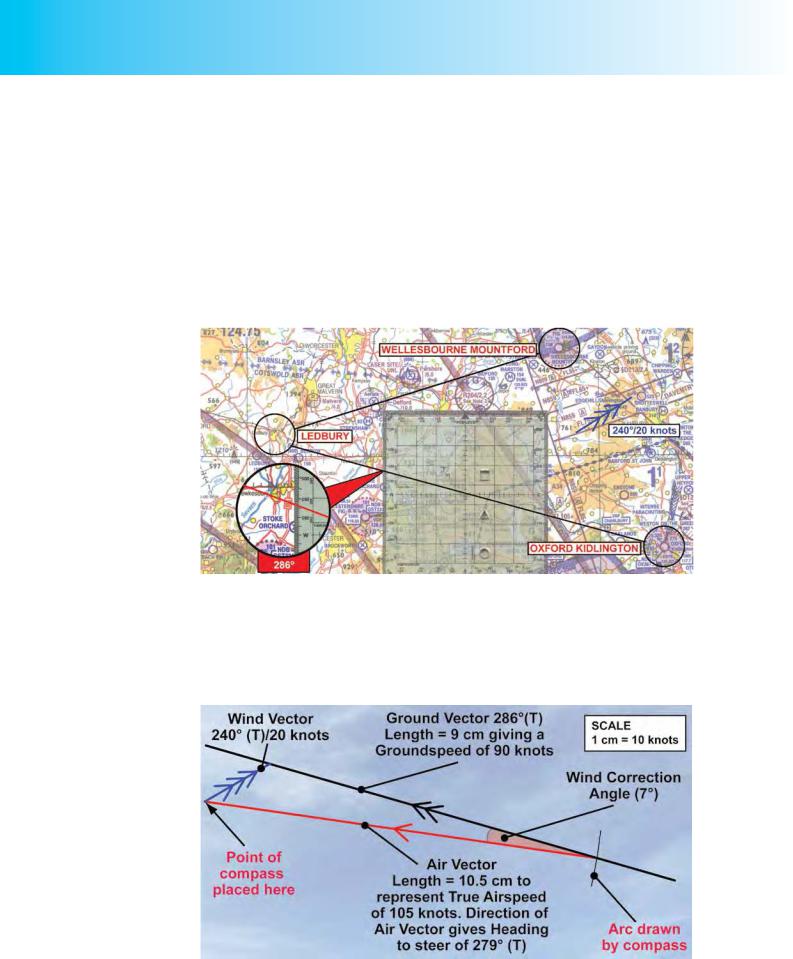
In order to illustrate how heading and groundspeed are calculated on the navigation computer, we will stay with our route from Oxford Kidlington to Wellesbourne Mountford, via Ledbury.

Figure 11.4 The route from Kidlington to Ledbury. The route is to be flown at 105 knots, True

Airspeed. What will be the True Heading and Groundspeed?

In Chapter 9, we worked out, using the triangle of velocities method, the heading that we need to fly from Oxford Kidlington to Ledbury, in order to make good the true track of 286°(T), at a true airspeed of 105 knots, in a wind from 240°(True), at 20 knots. You will remember that the heading and groundspeed were 279° (True), and 90 knots, respectively. (See Figure 11.5.)

Figure 11.5 The Triangle of Velocities constructed to determine True Heading and

Groundspeed on the route from Kidlington to Ledbury.

178

ID: 3658

Customer: Oleg Ostapenko E-mail: [e-mail]

Customer: Oleg Ostapenko E-mail: [e-mail]

CHAPTER 11: THE NAVIGATION COMPUTER

You will now learn how you carry out the same calculations for heading and groundspeed, but, this time, on the navigation computer.

There are, in fact, two ways of carrying out this calculation on the navigation computer. Both methods are taught on the CD-ROM. Here, we shall use the more straightforward of the two methods, known as the “wind-up method”. You should follow through the method we are about to teach you on your own navigation computer.

It is vitally important to be minutely accurate in your movement of the scales and your pencil marking.

On the wind face of your navigation computer rotate the inner scale in order to set the wind direction of 240° against the index mark at the top of the outer fixed scale.

Position any of the speed arcs on the slide, centrally, in the blue aperture in the middle of the rotating part of the wind face. We have used the 100 knots speed arc, but any arc will do. Following the vertical centre line of the slide, mark a point, with a sharp, soft pencil or chinagraph, 20 knots up from the arc under the blue aperture. You mark the point on the 120 knots speed arc, on the slide centre line. This point represents the 20 knots wind speed. You just need to mark the point, but we have drawn a wind vector line in our diagram, because the wind vector is what you have just marked on the computer. (See Figure 11.6.)

Figure 11.6 Marking the wind vector.

179

Order: 6026

Customer: Oleg Ostapenko E-mail: [e-mail]

Customer: Oleg Ostapenko E-mail: [e-mail]

CHAPTER 11: THE NAVIGATION COMPUTER

The method we are using is called the “wind up method” simply because we have marked the wind speed “up” from the blue aperture.

Now rotate the inner scale to set the desired track of 286°(T) against the index mark. The slide centre line now gives you the orientation of the ground vector, of the triangle of velocities.

Figure 11.7 Position the Desired Track against the Index Mark and adjust the slide to place the True Airspeed under the Wind Mark.

We have marked the ground vector on the wind face, but you do not need to do so. You should now be able to see the triangle of velocities taking shape with the wind vector pointing towards the ground vector, just as in real life, the wind will effectively blow the aircraft from its heading onto its track.

Now adjust the slide so that the speed arc representing the planned true airspeed of 105 knots is coincident with the wind mark. (See Figure 11.7.)

Note that the wind mark is now over the 7 degree drift line to the left of the centre line. (See Figure 11.8.) Using the “wind up method”, the drift lines indicate the direction in which we have to head our aircraft in order to compensate for drift. So, in this case, with the wind mark to the left of the centre line, we need to head left by 7°. Therefore,

180

ID: 3658

Customer: Oleg Ostapenko E-mail: [e-mail]

Customer: Oleg Ostapenko E-mail: [e-mail]

CHAPTER 11: THE NAVIGATION COMPUTER

we subtract 7° from the desired track of 286º(T) to obtain a true heading to steer of 279°(T). If the wind mark were to the right of the centre line, we would add drift to our track to obtain our heading.

From Figure 11.8, you can see that the navigation computer has now completed the construction of the triangle of velocities. Though you can not see the whole triangle, it is indeed complete, the drift line of 7° to port representing the air vector; that is the vector which gives us the heading to steer, based on our true airspeed.

Figure 11.8 The calculation of heading and groundspeed is complete.

The length of the ground vector is now represented by the speed arc which lies under the blue aperture. That speed arc gives us our groundspeed of 90 knots.

We have calculated, then, that at a true airspeed of 105 knots, with a wind from 240°

(True) at 20 knots, we need to fly a heading of 279° (True) to maintain a track of 286°

(True).

In order to find the heading to steer on your compass, do not forget to apply the local magnetic variation, and then to make any required deviation correction by consulting the compass deviation card. You will see that the values for heading to steer and groundspeed are identical to those that we obtained from the geometrically constructed triangle of velocities in Chapter 9.

181

Order: 6026

Customer: Oleg Ostapenko E-mail: [e-mail]

Customer: Oleg Ostapenko E-mail: [e-mail]

CHAPTER 11: THE NAVIGATION COMPUTER

Now try, yourself, to work out the heading to and groundspeed for the cross country leg from Ledbury to Wellesbourne Mountford. Our solution is printed in the partially completed flight log at Figure 9.15, in Chapter 9.

You will find numerous test calculations on heading and groundspeed on the CD-

ROM.

TRUE AIR SPEED.

As you learnt in Chapter 9, the value for airspeed which must be used for all navigational calculations is the aircraft’s true airspeed. The crucial consideration in navigational calculations is that airspeed should refer to the actual speed with which the aircraft is moving relative to the air mass in which it is flying. This is what we mean by true airspeed.

You learn in Chapter 9, and in the ‘Principles of Flight’ and ‘Aeroplanes’ volumes in this series of books, that when atmospheric conditions differ from ICAO Standard

Atmosphere (ISA) sea-level conditions, there is a significant difference between the indicated airspeed that the pilot reads from the Airspeed Indicator (ASI) and the aircraft’s true airspeed. All ASIs are calibrated with respect to ISA sea-level conditions.

Indicated airspeed is proportional to the dynamic pressure (Q), sensed by the ASI. The equation for dynamic pressure is Q = ½ ρv2. In this equation, v represents true airspeed and ρ represents air density. Therefore, for any given value of true airspeed, if ρdecreases, the indicated airspeed, as a function of Q, will also decrease. Consequently, as density decreases with increasing altitude, indicated airspeed, at altitude, will inevitably be lower than true airspeed. This error in the ASI reading is known as density error.

As you learn elsewhere, the atmospheric parameters which govern the value of density are pressure and temperature. Both pressure and temperature decrease with altitude. The navigation computer allows you to calculate true airspeed for any indicated airspeed, by entering values for the altitude at which you plan to fly, the temperature at that altitude and your planned indicated airspeed. (Note that the altitude for which you wish to calculate the true airspeed equivalent of any indicated airspeed must be pressure altitude; that is, altitude measured with respect to a pressure datum of 1013.2 millibars (hectopascals).)

The ASIs fitted to many aircraft may suffer from position and instrument errors.

Indicated airspeed corrected for these errors is known as calibrated airspeed or rectified airspeed. The Pilot’s Operating Manual will contain calibration tables to convert indicated airspeed readings into calibrated or rectified airspeed. For accurate conversions of the ASI reading to true airspeed, pilots should ideally use the calibrated or rectified airspeed. However, instrument and position errors on ASIs are often very small, so, for PPL light aircraft flying the indicated airspeed can usually be used as the basis for calculating true airspeed. This is the practice we shall adopt in this chapter. You learn more about indicated airspeed, calibrated or rectified airspeed and true airspeed in ‘Principles of Flight’ and ‘Aeroplanes’.

Calculating True Airspeed Using the Navigation Computer.

There follows an example of how true airspeed calculations are carried out using the navigation computer. There are more examples, as well as numerous test questions, on the CD-ROM.

182

ID: 3658

Customer: Oleg Ostapenko E-mail: [e-mail]

Customer: Oleg Ostapenko E-mail: [e-mail]

CHAPTER 11: THE NAVIGATION COMPUTER

Let us assume that we are planning to fly a route at 3000 feet on a fine day in

January in the United Kingdom, when the Regional Pressure Setting (RPS) for our area is given as 1003 millibars, and the temperature at 3000 feet is forecast to be +2°

Celsius (C). We plan to fly the route at an indicated airspeed of 110 knots. What will be the true airspeed that we need to use in order to calculate our heading and groundspeed for the route?

First of all we must express our chosen cruising altitude as a pressure altitude. As the atmospheric pressure at sea-level for our region (the RPS) is given as 1003 millibars, the datum of 1013.2 millibars, which we need for our true airspeed calculation, will lie lower than the RPS, and the pressure altitude will, therefore, be higher than 3000 feet. As pressure changes by about 1 millibar for every 30 feet of altitude, and the difference between 1003 millibars and 1013.2 millibars is, for all practical purposes, 10 millibars, we deduce that the pressure altitude equivalent of 3000 feet, on the day of our flight, will be 3000 + (30 x 10) = 3300 feet.

Now, on the circular slide-rule face of the navigation computer, identify the window marked Airspeed. The Airspeed window is depicted in Figure 11.9.

Figure 11.9 At 3300 ft pressure altitude with a temperature of +2°C, 110 knots indicated airspeed is the equivalent of 114 knots true airspeed.

183

Order: 6026

Customer: Oleg Ostapenko E-mail: [e-mail]

Customer: Oleg Ostapenko E-mail: [e-mail]

CHAPTER 11: THE NAVIGATION COMPUTER

Practise mental

calculations of Speed,

Distance and Time regularly. Skill at mental arithmetic is essential for the pilot-navigator.

The top moveable scale of the Airspeed window is the temperature in °C; the fixed scale inside the window is the pressure altitude in 1000s of feet. We, therefore, set the pressure altitude of 3300 feet against the forecast temperature at that altitude of 2°C, as depicted in Figure 11.9. Setting up these figures requires a bit of estimation between scale gradations, so use the computer’s cursor to help you. Set the cursor line over your best estimate for 3300 feet and then line up +2°C with the cursor, too. With the circular slide rule set up in this way, true airspeed can be read off on the slide rule’s outer scale against the indicated airspeed on the inner scale. Against our planned indicated airspeed of 110 knots on the inner scale, we read off, on the outer scale, the equivalent true airspeed of 114 knots.

As a rough approximation, true airspeed is about 8% more than indicated airspeed at

5000 feet, and 17% greater at 10 000 feet, so 114 knots seems a reasonable figure for 3300 feet, being 4% greater than 110 knots.

114 knots true airspeed will be the airspeed figure that we use in our navigation calculations for our planned flight.

If you wish to practise more true airspeed conversions, there are many more on the CD-ROM.

SPEED, DISTANCE & TIME CALCULATIONS.

Introduction.

In Chapter 4, you learnt about the importance of speed, distance & time calculations to the pilot-navigator. You learnt, too, that in carrying out these calculations it is of crucial importance that the units match one another, otherwise you will obtain nonsense answers. Revise Chapter 4 now, if you feel it to be necessary.

In this section on the navigation computer, you will learn how to use the computer to carry out speed, distance and time calculations much more quickly and easily than is possible when working them out “long-hand”, or in your head.

You should, nevertheless, get used to working out estimates of speed, distance & time calculations mentally, and practise mental calculation regularly, as a means of checking the order of magnitude of the solutions obtained from the navigation computer. It cannot be over-emphasised how important it is for you to know where to place the decimal point in the figures that you read off from the various scales on the computer. For instance, if you were to read off, as a solution to a particular problem, the figures 185, you will know where to place the decimal point in these figures only if you have calculated mentally the order of magnitude of the answer. Are you expecting an answer of 185, 18.5, 1.85, 0.185, 0.0185?

Calculating Time.

During the flight planning stage of a cross country trip, after calculating your heading to steer and groundspeed for each leg, you will need to work out the time required for each leg, as well as the time required for the whole trip, in order that you can work out your fuel requirements.

Timings are entered in the flight log, along with the fuel requirements for the whole trip, as well as the fuel required to complete the flight from nominated turning points and checkpoints, based on your aircraft’s fuel consumption rate.

184

ID: 3658

Customer: Oleg Ostapenko E-mail: [e-mail]

Customer: Oleg Ostapenko E-mail: [e-mail]

CHAPTER 11: THE NAVIGATION COMPUTER

As an example of carrying out time calculations on the navigation computer, let us calculate the time required to fly from Oxford Kidlington to Wellesbourne Mountford, via, Ledbury, based on the groundspeed for the two legs of that flight, that we worked out earlier. We have, in fact, already worked out the times, long hand, and entered them in the flight log, in Figure 9.15, but we will now show you how to work out those times on the navigation computer.

Time Required for the Leg from Oxford Kidlington to Ledbury.

We have already measured the distance and calculated the groundspeed for the leg from Oxford Kidlington to Ledbury. The distance is 42 nautical miles (nm), and the groundspeed worked out to be 90 knots.

We know that time	=		distance
			groundspeed

Distance is in nm, and groundspeed is in knots (i.e. nm per hour), so the units match. The navigation computer permits you to read off the time in minutes or hours and minutes.

On the navigation computer, the index mark we use for speed, distance, time calculations is the 60 index, on the inner scale. (With speed, distance & time, we are working in hours, minutes and seconds, so we are working to base 60, not base 10.)

In order to calculate the time required to cover a given distance at a given groundspeed, simply position the 60 index on the inner scale against groundspeed on the outer scale. For the first leg of the flight from Oxford Kidlington to Ledbury, the calculated groundspeed is 90 knots, so we set the 60 index against 90 on the outer scale.

With the 60 index on the inner scale against the value of 90 on the outer scale, any distance you require can be identified on the outer scale and the resulting time required, in minutes, or in hours and minutes, to cover that distance at the selected groundspeed may be read from the two inner scales. Note that the blue inner scale has numbers only; these are read off as minutes. The white inner scale, inside the blue scale, indicates hours and minutes. It is essential, therefore, that you carry out an approximate mental calculation of the time that you are expecting, so that you know whether to expect a time in minutes, or in hours and minutes.

In this case, you position the cursor over 42 (for 42 nm) on the outer scale and as illustrated in Figure 11.10, you see that the corresponding value on the inner scale is almost exactly 28.

Now you will see the importance of carrying out approximate mental calculations. You need to have worked out mentally that at 90 knots (90 nm per hour) it will take less than an hour to cover 42 nm. In fact, it is fairly easy to work out in your head that at a groundspeed of 90 knots, an aircraft will cover 42 nautical miles in just less than ½ an hour. Therefore, you should easily deduce that the value 28 represents

28 minutes. You, therefore, enter a time of 28 minutes in the flight log for the leg from Oxford Kidlington to Ledbury. You will see that this is exactly the same time as that which we calculated earlier, with pencil and paper. All calculations are as straightforward as that, really.

185

Order: 6026

Customer: Oleg Ostapenko E-mail: [e-mail]

Customer: Oleg Ostapenko E-mail: [e-mail]

CHAPTER 11: THE NAVIGATION COMPUTER

Figure 11.10 Calculating the time taken to fly 42 nm at a groundspeed of 90 knots.

Remember, you are using the 60 index, so any time indicated by the blue inner scale will be in minutes. The white inner scale gives answers in hours and minutes, if the solution is greater than one hour.

Without moving the 60 index from its position against 90 knots, you can now read off the expected elapsed time from Oxford Kidlington to your first checkpoint at Little

Rissington, 14 nm along the route. That will be 9½ minutes.

Similarly, the elapsed time from Oxford Kidlington to the second checkpoint of the M5, at 32 nm distance, can be read off the inner scale of the navigation computer as 21 minutes, to the nearest minute.

Time Required for the Leg from Ledbury to Wellesbourne Mountford.

We measured the leg from Ledbury to Wellesbourne Mountford to be 32 nm and calculated that in the prevailing wind we would make a groundspeed of 125 knots. In order, then, to calculate the time required for the leg, we position the 60 index against 125 on the outer scale, identify the value 32 (for the distance of 32 nm) on the outer scale, and read off the value 153 from the divisions on the blue inner scale, as illustrated in Figure 11.11.

186