Maxwell v15		6.3
	Eddy Current – Application Note

Create a Plot of Force vs. Time

The time-averaged, AC, and instantaneous components Lorentz force can be plotted vs. time by creating named expressions in the calculator using the formulas at the beginning of the application note.

1.Determine the time-averaged component of Lorentz force:

•Click on Maxwell 3D > Fields > Calculator and then perform the following:

•Quantity > J

•Quantity > B > Complex > Conj > Cross

•Scalar Y > Complex > Real

•Number > Scalar > 0.5 > OK

•Multiply

•Geometry > Volume > left > OK

•Integrate

•Add… Name: Force_DC

•OK

2.Determine the AC component of Lorentz force:

•Quantity > J

•Quantity > B > Cross

•Scalar Y

•Function > Phase > OK

•Complex > AtPhase

•Number > Scalar > 0.5 > OK

•Multiply

•Geometry > Volume > left > OK

•Integrate

•Add… Name: Force_AC

•OK

3.Determine the instantaneous (DC + AC) component of Lorentz force. In the Named Expressions panel:

•In the Named Expressions window, select Force_DC and Copy to stack

•Select Force_AC and Copy to stack

•Add

•Add… Name: Force_inst

•Click on OK and Done to close the calculator window.

ANSYS Maxwell Field Simulator v15 User’s Guide

6.3 - 14

Maxwell v15		6.3
	Eddy Current – Application Note

4.Create a plot of Force vs. Phase. Now that the force quantities have been created, a plot of these named expressions can been created.

•Select Maxwell 3D > Results > Create Fields Report > Rectangular Plot

•Category: Calculator Expressions

•Change the Primary Sweep: from the default Freq to Phase.

•Quantity: Force_DC, Force_AC, Force_inst (hold down shift key to select all three at once)

•New Report > Close

•Right mouse click on the legend and select: Trace Characteristics > Add…

•Category: Math

•Function: Max

•Add > Done

•Double left mouse click on the legend and change from the Attribute to the General tab.

•Check Use Scientific Notation and click on OK. Note that these values match the results on the Solution Data > Force. Also, since forces fluctuate at 2 times the excitation frequency, there are two complete cycles in 360 degrees shown below.

This completes PART 2 of the exercise.

Reference:

MSC Paper #118 "Post Processing of Vector Quantities, Lorentz Forces, and Moments

in AC Analysis for Electromagnetic Devices" MSC European Users Conference, September 1993, by Peter Henninger, Research Laboratories of Siemens AG, Erlangen

ANSYS Maxwell Field Simulator v15 User’s Guide

6.3 - 15

	Maxwell v15		7.0
	Chapter 7.0 – Magnetic Transient

Chapter 7.0 – Magnetic Transient

7.1 – Switched Reluctance Motor (Stranded Conductors)

7.2 – Rotational Motion

7.3 – Translational Motion

7.4 – Core Loss

ANSYS Maxwell 3D Field Simulator v15 User’s Guide							7.0

Maxwell v15

7.1

Example (Transient) – Stranded Conductors

Stranded Conductors

This example is intended to show you how to create and analyze a transient problem on a Switched Reluctance Motor geometry using the Transient solver in the Ansoft Maxwell 3D Design Environment.

Within the Maxwell 3D Design Environment, solid coils can be modeled as Stranded Conductors. There are many advantages to using Stranded Conductors when modeling coils that have multiple turns. The first obvious advantage is that a coil with multiple wires, say 2500, can be modeled as a single object as opposed to modeling each wire which would be impracticable. Defining a Stranded Conductor means that the current density will be uniform throughout the cross section of the conductor.

The example that will be used to demonstrate how Stranded Conductors are implemented is a switched Reluctance Motor. This switched reluctance motor will have four phases and two coils per phase, thus we can show how independent coils can be grouped to create windings.

Note: This tutorial shows how to setup a stranded conductor using Transient Solver and does not involve details regarding geometry creation. To see geometry creation details, please refer the example 5.3

ANSYS Maxwell 3D Field Simulator v15 User’s Guide			7.1-1

Maxwell v15

7.1

Example (Transient) – Stranded Conductors

Theory – Transient Solver

When creating Windings in the Transient solver, it is assumed that all of the coils used to make up that winding are connected in series.

When creating a Winding and using voltage sources, the Winding Panel asks for the Initial Current, Resistance, Inductance, and Voltage.

Initial Current: This is an initial condition used by the solver

Resistance: This is the DC resistance of the total winding; for the Phase_A winding, this is the resistance of Coil_A1 and Coil_A2 in series.

Inductance: This is any extra inductance that is not modeled that needs to be added. For example, and additional line inductance or source inductance.

Voltage: This is the source voltage which can be a constant, function, or piecewise linear curve.

A sketch of the Phase_A Winding circuit is:

ANSYS Maxwell 3D Field Simulator v15 User’s Guide					7.1-2

Maxwell v15

7.1

Example (Transient) – Stranded Conductors

Theory – Transient Solver (Continued)

If the Winding was defined as a Current Source instead of a Voltage Source, the only additional field to modify is the initial current. The circuit would look like this:

The DC Resistance and Extra Inductance is not needed since this is a current source and its value is guaranteed regardless of any value for the DC Resistance or Extra Inductance.

The third option for the Winding setup is External. This means that there is an external circuit that is made up of arbitrary components. Please refer to the Topic paper on External Circuits for the details on how this is implemented.

Please note that if the two coils that make up the Phase_A winding were connected in parallel instead of series, then two separate Windings would need to be created.

In regards to the current density, the Transient solver treats stranded conductors the same as in the Magnetostatic solver; that is, the current density is uniform across the terminal and the solver calculates the magnetic field intensity H directly and the current density vector J indirectly.

There are two options when defining the type of winding: Solid or Stranded. This write up is for Stranded Windings only. For a full description of how Solid windings are implemented, please refer to the Topic paper Solid Conductors.

ANSYS Maxwell 3D Field Simulator v15 User’s Guide					7.1-3

Maxwell v15

7.1

Example (Transient) – Stranded Conductors

ANSYS Maxwell Design Environment

The following features of the ANSYS Maxwell Design Environment are used to

create the models covered in this topic

3D Solid Modeling

Boolean Operations: Split

Boundaries/Excitations

Current: Stranded

Analysis

Transient

Results

Field Calculator

Field Overlays:

Magnitude B

ANSYS Maxwell 3D Field Simulator v15 User’s Guide					7.1-4

Maxwell v15

7.1

Example (Transient) – Stranded Conductors

Launching Maxwell

To access Maxwell:

1.Click the Microsoft Start button, select Programs, and select Ansoft > Maxwell 15.0 and select Maxwell 15.0

Setting Tool Options

To set the tool options:

Note: In order to follow the steps outlined in this example, verify that the following tool options are set :

1. Select the menu item Tools > Options > Maxwell 3D Options

Maxwell Options Window:

1. Click the General Options tab

Use Wizards for data input when creating new boundaries:  Checked

Duplicate boundaries/mesh operations with geometry:

Checked

2.Click the OK button

2.Select the menu item Tools > Options > Modeler Options.

Modeler Options Window:

1. Click the Operation tab

Automatically cover closed polylines:  Checked 2. Click the Display tab

Default transparency = 0.8 3. Click the Drawing tab

Edit property of new primitives:  Checked 4. Click the OK button

ANSYS Maxwell 3D Field Simulator v15 User’s Guide					7.1-5

Maxwell v15

7.1

Example (Transient) – Stranded Conductors

Open Existing File

To Open a File

Select the menu item File > Open

Locate the file Ex_5_3_Stranded_Conductors.mxwl and Open it

Set Solution Type

To set the Solution Type:

Select the menu item Maxwell 3D > Solution Type

Solution Type Window:

1.Choose Magnetic > Transient

2.Click the OK button

Save File

To Save File

Select the menu item File > Save

Save the file with a name Ex_7_1_Transient_Reluctance_Motor

DeleteExcitations

Delete Specified Excitations

As we have opened the file from a Magnetostatic setup, the excitation are already existing in the file

Delete all excitations from Project Manager tree as new excitations will be specified according to Transient Solver

ANSYS Maxwell 3D Field Simulator v15 User’s Guide			7.1-6

Maxwell v15

7.1

Example (Transient) – Stranded Conductors

Specify Coil Terminals

To Specify Coil terminals

Expand the history tree for Sheets

Press Ctrl and select the all sheet objects

Select the menu item Maxwell 3D > Excitations > Assign > Coil Terminal

In Coil Terminal Excitation window,

1.Base Name: CoilTerminal

2.Number of Conductors: 150

3.Press OK

Specify Windings

To Add Winding

Select the menu item Maxwell 3D > Excitations > Add Winding

In Winding window,

1.Name: Winding1

2.Type: Voltage

3.Stranded:  Checked

4.Initial Current: 0 A

5.Resistance: 2.3 ohm

6.Inductance: 0 mH

7.Voltage: 120 V

8.Press OK

ANSYS Maxwell 3D Field Simulator v15 User’s Guide			7.1-7

Maxwell v15

7.1

Example (Transient) – Stranded Conductors

Add Terminals to Winding

Expand the Project tree to display terminals

Right click on the Winding1 from the Project tree and select Add Terminals In Add Terminals window,

1.Press Ctrl and select the terminals CoilTerminal_1 and CoilTerminal_2

2.Press OK

Repeat the same steps to three more windings

Winding2

CoilTerminal_3

CoilTerminal_4

Winding3

CoilTerminal_5

CoilTerminal_6

Winding4

CoilTerminal_7

CoilTerminal_8

Assign Mesh Operations

Note: The transient solver does not use automatic adaptive meshing.

Assign Mesh Operations for Coils

Press Ctrl and select all the object corresponding to coils from history tree

Select the menu item Maxwell 3D > Mesh Operations > Assign > Inside Selection > Length Based

In Element Length Based Refinement window,

1.Restrict Length of Elements:  Unchecked

2.Restrict the Number of Elements:  Checked

3.Maximum Number of Elements: 16000 (2000/tets per coil)

4.Click the OK button

ANSYS Maxwell 3D Field Simulator v15 User’s Guide					7.1-8

Maxwell v15

7.1

Example (Transient) – Stranded Conductors

Assign Mesh Operations for Stator and Rotor

Press Ctrl and select the objects Stator and Rotor from the history tree

Select the menu item Maxwell 3D > Mesh Operations > Assign > Inside Selection > Length Based

In Element Length Based Refinement window,

1.Restrict Length of Elements:  Unchecked

2.Restrict the Number of Elements:  Checked

3.Maximum Number of Elements: 4000 (2000/tets per object)

4.Click the OK button

Analysis Setup

To create an analysis setup:

Select the menu item Maxwell 3D > Analysis Setup > Add Solution Setup

Solution Setup Window:

1. Click the General tab:

Stop time: 0.02s Time step: 0.002s

2. Click the OK button

Model Validation

To validate the model:

Select the menu item Maxwell 3D > Validation Check

Click the Close button

Note: To view any errors or warning messages, use the Message Manager.

Analyze

To start the solution process:

1. Select the menu item Maxwell 3D > Analyze All

ANSYS Maxwell 3D Field Simulator v15 User’s Guide			7.1-9

Maxwell v15

7.1

Example (Transient) – Stranded Conductors

Create Quick Report

To Create a Report

Select the menu item Maxwell 3D > Results > Create Transient Reports > Rectangular Plot

In Report Window,

1.Category: Winding

2.Quantity: Press Ctrl and select Current(Winding1), Current(Winding2), Current(Winding3), Current(Winding4)

3.Select the button New Report

4.Press Close

Right Click on the plot and select Trace Characteristics > Add

In Add Trace Characteristics window,

Category: Math

Function: Max

Select Add and Done

ANSYS Maxwell 3D Field Simulator v15 User’s Guide					7.1-10

Maxwell v15

7.1

Example (Transient) – Stranded Conductors

Calculate Current

To Calculate Current

Select the menu item Maxwell 3D > Fields > Calculator

In Fields Calculator window,

1.Select Input > Quantity > J

2.Select Vector: Scal? > Scalar Z

3.Select Input > Geometry

Set the radio button to Surface

From the list select Terminal_A1

Press OK

4.Select Scalar > ∫ (Integrate)

5.Select Input > Number

Type: Scalar

Value: 150 (Number of Conductors)

Press OK

6.Select General > /

7.Select Output > Eval

8.Press Done to close the calculator

Note that the value reported in calculator is same as the value shown in plot in the last step

ANSYS Maxwell 3D Field Simulator v15 User’s Guide			7.1-11

Maxwell v15

7.1

Example (Transient) – Stranded Conductors

Create Quarter Symmetry Geometry

So far we have been working with full geometry. Often it is useful to use symmetry in order to reduce the problem size and thus decrease the solution time. In this section, we’ll show how to create the symmetric model and its impact on stranded conductors.

Create Symmetry Design

Copy Design

Select the design Maxwell3DDesign1 in Project Manager window, right click and select Copy

Select project Ex_7_1_transient_reluctance_motor in Project Manager window and select Paste

Rotatethe Geometry to Create Quarter Symmetry

Before splitting the model to create a ¼ model, all of the objects need to be rotated.

To Rotate Model

Select the menu item Edit > Select All

Select the menu item Edit > Arrange > Rotate

In Rotate Window,

1.Axis: Z

2.Angle: 22.5 deg

3.Press OK

To Rotate the object Rotor

Select the object Rotor from the history tree

Select the menu item Edit > Arrange > Rotate

In Rotate Window,

1.Axis: Z

2.Angle: 7.5 deg

3.Press OK

ANSYS Maxwell 3D Field Simulator v15 User’s Guide			7.1-12

Maxwell v15

7.1

Example (Transient) – Stranded Conductors

Split Model

Divide by XY Plane

Select the menu item Edit > Select All

Select the menu item Modeler > Boolean >Split

In Split window

1.Split plane: XY

2.Keep fragments: Positive side

3.Split objects: Split entire selection

4.Press OK

Divide by YZ Plane

Select the menu item Edit > Select All

Select the menu item Modeler > Boolean >Split

In Split window

1.Split plane: YZ

2.Keep fragments: Negative side

3.Split objects: Split entire selection

4.Press OK

ANSYS Maxwell 3D Field Simulator v15 User’s Guide			7.1-13

Maxwell v15

7.1

Example (Transient) – Stranded Conductors

Redefining the Terminals

When the entire coil is not being modeled and the coil cuts the surface of the solution boundary (called Region in this example), terminals need to be defined that are coincident with the Coil and the Region.

To Redefine Terminals

Press Ctrl and select the objects Region, Stator and Rotor

Select the menu item View > Visibility > Hide Selection > Active View

Select the menu item Edit > Select > Faces

Select the face of Coil_A2 that coincides with region as shown in below image

Select the menu item Maxwell 3D > Excitations > Assign > Coil Terminal

In Coil Terminal Excitation window,

1.Name: Terminal_A2_1

2.Number of Conductors: 150

3.Press OK

Select the other face of the object Coil_A2 that touches with region

Select the menu item Maxwell 3D > Excitations > Assign > Coil Terminal

In Coil Terminal Excitation window,

1.Name: Terminal_A2_2

2.Number of Conductors: 150

3.Press the button Swap Direction to invert current direction

4.Press OK

ANSYS Maxwell 3D Field Simulator v15 User’s Guide							7.1-14

Maxwell v15

7.1

Example (Transient) – Stranded Conductors

Redefine coil terminals as specified in below image for other objects

Ensure the direction of current is consistent in all coils.

Add Terminals to Windings

To Add Terminals

Right click on Winding1 which exists from previous settings and select Add Terminals

In Add Terminals window,

1.Press Ctrl and select the terminals Terminal_A2_1 and Terminal_A2_2

2.Press OK

Repeat the same steps to three more windings

Winding2

Terminal_B1_1, Terminal_B1_2, Terminal_B2_1, Terminal_B2_2

Winding3

Terminal_C1_1, Terminal_C1_2

Winding4

Terminal_D1_1, Terminal_D1_2

ANSYS Maxwell 3D Field Simulator v15 User’s Guide			7.1-15

Maxwell v15

7.1

Example (Transient) – Stranded Conductors

Modify Mesh Operations

To Modify Mesh Operations

Expand the Project Manager tree to view Mesh Operations

Double click on the mesh operation Length1 that corresponds to Coils In Element Length Based Refinement window,

1.Change Maximum Number of Elements to 4000 (1/4th of the value used for Full Model

2.Press OK

Double click on Length2 that corresponds to Stator and Rotor

In Element Length Based Refinement window,

1.Change Maximum Number of Elements to 1000 (1/4th of the value used for Full Model

2.Press OK

Set Symmetry Multiplier

To Set Symmetry Multiplier

Select the menu item Maxwell 3D > Model > Set Symmetry Multiplier

Set Symmetry Multiplier value of 4 in the window Press OK

Model Validation

To validate the model:

Select the menu item Maxwell 3D > Validation Check

Click the Close button

Note: To view any errors or warning messages, use the Message Manager.

Analyze

To start the solution process:

1. Select the menu item Maxwell 3D > Analyze All

ANSYS Maxwell 3D Field Simulator v15 User’s Guide			7.1-16

Maxwell v15

7.1

Example (Transient) – Stranded Conductors

Results

To View Results

Expand the Project Manager tree to view XY Plot 1 under Results

Create Sheet Object for Current Calculation

Select any of the end faces of Coil_A2

Select the menu item Modeler > List > Create > Face List

To Calculate Current

Select the menu item Maxwell 3D > Fields > Calculator

In Fields Calculator window,

1.Select Input > Quantity > J

2.Select Vector: Scal? > Scalar Z

3.Select Input > Geometry

Set the radio button to Surface

From the list select Facelist1

Press OK

4.Select Scalar > ∫ (Integrate)

5.Select Input > Number

Type: Scalar

Value: 150 (Number of Conductors)

Press OK

6.Select General > /

7.Select Output > Eval

8.Press Done to close the calculator

The value of current is around 52 A which is save as previous

ANSYS	Maxwell 3D Field Simulator v15 User’s Guide	7.1-17

Maxwell v15

7.1

Example (Transient) – Stranded Conductors

Half Coils

Note: If the cross section of the coil is cut in half, then the number of conductors is half. An example for a simple coil is shown below:

H = 20mm

H = 10mm

Modeling the Full Coil:

Cut the Full Coil in half and use an

Conductor Number = 150

Odd Symmetry Boundary:

Symmetry Multiplier = 1

Conductor Number = 75

ANSYS Maxwell 3D Field Simulator v15 User’s Guide			7.1-18

Maxwell v15

7.2

Example (Transient) – Rotational Motion

Rotational Cylindrical Motion using the Transient Solver

Transient Solver in Maxwell allows to be combined with motion. This motion can be translational, rotational cylindrical or rotational non-cylindrical (relay-type motion). This example shows on a simple geometry how to set-up rotational cylindrical motion project in a Transient Solver. It teaches how to set-up a band for rotational cylindrical motion, create and post process time-dependent field variables and create an animation. It shows how to utilize the periodicity of the configuration to reduce the size of the problem.

The geometry consists of a cylindrical 4-pole radially magnetized NdFeB magnet with sinusoidal distribution of magnetization. The magnet rotates with a constant speed of 360 degrees per second around its axis. There is a Hall Sensor at certain distance from the magnet. The goal is to model a time-dependent magnetic field created by rotating magnet and follow the magnitude of this field by employing the Hall sensor. The role of the sensor is to calculate the average flux density passing through the sensor.

ANSYS Maxwell 3D Field Simulator v15 User’s Guide			7.2-1

Maxwell v15

7.2

Example (Transient) – Rotational Motion

ANSYS Maxwell Design Environment

The following features of the ANSYS Maxwell Design Environment are used to create the models covered in this topic

3D Solid Modeling

Primitives: Regular Polyhedron, Rectangle

Boolean Operations: Split

Sweep Operations: Around Axis

Model: Band for rotational cylindrical motion

Boundaries/Excitations

Matching boundaries (Master/Slave)

Natural outer boundary

Material properties

Edit material (4-pole NdFeB radially magnetized magnet)

Analysis

Transient

Results

Fields Calculator

Rectangular Plot

Field Overlays:

Flux Density Vector Plots Flux Density Vector Animation

ANSYS Maxwell 3D Field Simulator v15 User’s Guide					7.2-2

Maxwell v15

7.2

Example (Transient) – Rotational Motion

Launching Maxwell

To access Maxwell:

1.Click the Microsoft Start button, select Programs, and select Ansoft > Maxwell 15.0 and select Maxwell 15.0

Setting Tool Options

To set the tool options:

Note: In order to follow the steps outlined in this example, verify that the following tool options are set :

1. Select the menu item Tools > Options > Maxwell 3D Options

Maxwell Options Window:

1. Click the General Options tab

Use Wizards for data input when creating new boundaries:  Checked

Duplicate boundaries/mesh operations with geometry:

Checked

2.Click the OK button

2.Select the menu item Tools > Options > Modeler Options.

Modeler Options Window:

1. Click the Operation tab

Automatically cover closed polylines:  Checked 2. Click the Display tab

Default transparency = 0.8 3. Click the Drawing tab

Edit property of new primitives:  Checked 4. Click the OK button

ANSYS Maxwell 3D Field Simulator v15 User’s Guide					7.2-3

Maxwell v15

7.2

Example (Transient) – Rotational Motion

Opening a New Project

To open a new project:

After launching Maxwell, a project will be automatically created. You can also create a new project using below options.

1.In an Maxwell window, click the  On the Standard toolbar, or select the menu item File > New.

Select the menu item Project > Insert Maxwell 3D Design, or click on the icon

Set Solution Type

To set the Solution Type:

Select the menu item Maxwell 3D > Solution Type

Solution Type Window:

1.Choose Magnetic > Transient

2.Click the OK button

ANSYS		Maxwell 3D Field Simulator v15 User’s Guide							7.2-4

Maxwell v15

7.2

Example (Transient) – Rotational Motion

Create Magnet

Two different ways can be used to create the magnet

Using primitives from menu item Draw > Cylinder

Create a rectangle and sweep it along an axis

Here we will use second approach

To Create Rectangle

Select the menu item Modeler > Grid Plane > XZ

Select the menu item Draw > Rectangle

1. Using Coordinate entry field, enter the position of rectangle

X = 5, Y = 0, Z = -1, Press the Enter key

2. Using Coordinate entry field, enter the opposite corner of rectangle

X = 7, Y = 0, Z = 1, Press the Enter key (Note: Above values are in Absolute coordinates)

To Change Attributes

Select the resulting sheet from the history tree and goto Properties window

1.Change the name of the sheet to Magnet

2.Change the color of the sheet to Blue

To Sweep Rectangle

Select the sheet Magnet from the history tree

Select the menu item Draw > Sweep > Around Axis

In Sweep Around Axis window,

1.Sweep Axis: Z

2.Angle of Sweep: 360 deg

3.Press OK

ANSYS Maxwell 3D Field Simulator v15 User’s Guide							7.2-5

Maxwell v15

7.2

Example (Transient) – Rotational Motion

Create Hall Sensor

To Create Rectangle

Select the menu item Modeler > Grid Plane > YZ

Select the menu item Draw > Rectangle

1. Using Coordinate entry field, enter the position of rectangle

X = 8, Y = -0.4, Z = -0.4, Press the Enter key

2. Using Coordinate entry field, enter the opposite corner of rectangle

dX = 0, dY = 0.8, dZ = 0.8, Press the Enter key

To Change Attributes

Select the resulting sheet from the history tree and goto Properties window

1.Change the name of the sheet to Sensor

2.Change the color of the sheet to Red

To Rotate the Sheet

Select the sheet Sensor from the history tree

Select the menu item Edit > Arrange > Rotate

In Rotate window,

1.Axis: Z

2.Angle: 45 deg

3.Press OK

ANSYS Maxwell 3D Field Simulator v15 User’s Guide							7.2-6

Maxwell v15

7.2

Example (Transient) – Rotational Motion

Create Band

In a Transient Solver, Band is an object that contains all rotating objects. It is a way to tell Maxwell which objects are steady and which are moving. In this example there is one moving (rotating) object: Magnet. For rotational cylindrical type of motion Band is usually a cylinder or polyhedron. It should be a solid cylinder, not a hollow cylinder. For translational type of motion Band cannot be a true surface object (cylinder). It must be a faceted object, such as Regular Polyhedron.

To Create a Band Object

Select the menu item Modeler > Grid Plane > XY

Select the menu item Draw > Cylinder

1. Using Coordinate entry field, enter the center of base

X = 0, Y = 0, Z = -6, Press the Enter key

2. Using Coordinate entry field, enter the radius and height

dX = 7.3, dY = 0, dZ = 12, Press the Enter key

To Change Attributes

Select the resulting object from the history tree and goto Properties window

1.Change the name of the object to Band

2.Change the transparency of the object to 0.8

3.Change the color of the object to Brown

ANSYS Maxwell 3D Field Simulator v15 User’s Guide							7.2-7

Maxwell v15

7.2

Example (Transient) – Rotational Motion

Assign Material: Magnet

To Assign Magnet Material

Select the object Magnet from the history tree, right click and select Assign Material

In Select Definition window,

1.Type NdFe30 in the Search by Name field

2.Select option Clone Material

In View/Edit Material window,

1.Name: Magnet_Material

2.Material Coordinate System Type: Cylindrical

Note: The magnet is radially magnetized so it is advantageous to use the cylindrical coordinate system. The direction of magnetization is determined by Unit Vector. For the cylindrical coordinate system the components of Unit Vector are R, Phi and Z, standing for radial, circumferential and z- directions.

3. Magnetic Coercivity:

Magnitude: -838000

R Component: cos(2*Phi)

Note: Phi is a default symbol for an angle in cylindrical coordinate system. In order to get 4-pole magnet the argument in cos is multiplied by two.

4.Select Validate Material

5.Press OK

ANSYS Maxwell 3D Field Simulator v15 User’s Guide			7.2-8

Maxwell v15

7.2

Example (Transient) – Rotational Motion

Specify Motion

To Specify Band

Select the object Band from the history tree

Select the menu item Maxwell 3D > Model > Motion Setup > Assign Band

In Motion Setup window, 1. Type tab

Motion Type: Rotational

Rotation Axis: Global:Z

Positive 2. Mechanical tab

Angular Velocity: 360 deg_per_sec 3. Press OK

Create Region

To Create Region

Select the menu item Draw > Cylinder

1. Using Coordinate entry field, enter the center of base

X = 0, Y = 0, Z = -8, Press the Enter key

2. Using Coordinate entry field, enter the radius and height

dX = 16, dY = 0, dZ = 16, Press the Enter key

To Change Attributes

Select the resulting sheet from the history tree and goto Properties window

1.Change the name of the object to Region

2.Change Display Wireframe to  Checked

ANSYS Maxwell 3D Field Simulator v15 User’s Guide							7.2-9

Maxwell v15

7.2

Example (Transient) – Rotational Motion

Assign Mesh Operations

Transient solver does not use Adaptive meshing as for other solvers. Hence mesh parameters need to be specified in order to get refined mesh.

As we have defined Band region, Maxwell will automatically create a mesh operation in order to resolve cylindrical gap region between Band and the object inside it (Magnet). For rest, we need to manually specify mesh operations.

To Assign Mesh Operations for Magnet

Select the object Magnet from the history tree

Select the menu item Maxwell 3D > Mesh Operations > Assign > Inside Selection > Length Based

In Element Length Based Refinement window,

1.Name: magnet

2.Restrict Length of Elements:  Unchecked

3.Restrict the Number of Elements:  Checked

4.Maximum Number of Elements: 1000

5.Press OK

To Assign Mesh Operations for Region

Repeat the steps same as for Magnet and specify parameters as below

1.Name: region

2.Maximum Number of Elements: 8000

ANSYS Maxwell 3D Field Simulator v15 User’s Guide					7.2-10

Maxwell v15

7.2

Example (Transient) – Rotational Motion

To Assign Mesh Operations for Band

Since a cylinder is a true (curved) surface object, we will use Surface Approximation in order to create a good mesh for this rotational motion problem

Select the object Band from the history tree

Select the menu item Maxwell 3D > Mesh Operations > Assign > Surface Approximation

In Surface Approximation window,

1.

2.

Name: band

Maximum Surface Normal Deviation

Set maximum normal deviation (angle) : 3 deg

3. Maximum Aspect Ratio

Set aspect ratio: 5

4. Press OK

ANSYS Maxwell 3D Field Simulator v15 User’s Guide					7.2-11

Maxwell v15

7.2

Example (Transient) – Rotational Motion

Analysis Setup

To Create Analysis Setup

Select the menu item Maxwell 3D > Analysis Setup > Add Solution Setup

In Solve Setup Window, 1. General tab

Stop time: 1 s

Time step: 0.05 s

Note: We will analyze one revolution. Since the speed is 360 degrees per second, to analyze one revolution, we have to solve 1 s in time. We will discretize the time domain into 20 time steps, meaning that the time step will be 0.05 s

2. Save Fields tab

Type: Linear Step

Start: 0 s

Stop: 1 s

Step Size: 0.05 s

Select the button Add to List >> 3. Press OK

Save

To Save File

Select the menu item File > Save

Save the file with the name “Ex_7_2_Rotational_Motion.mxwl”

Analyze

To Run Solution

Select the menu item Maxwell 3D > Analyze All

ANSYS	Maxwell 3D Field Simulator v15 User’s Guide					7.2-12

Maxwell v15

7.2

Example (Transient) – Rotational Motion

Plot Flux Density Vector on XY plane at time 0 s

To Plot Flux Density at Time = 0 s

Select the menu item View > Set Solution Context

In Set View Context window,

1.Set Time to 0s

2.Press OK

Expand history tree for Planes and select Global:XY

Select the menu item Maxwell 3D > Fields > Fields > B > B_Vector

In Create Field Plot window, 1. Press Done

To Modify Plot Attributes

Double click on the legend to modify plot

In the window,

1. Marker/Arrow tab

Size: Set to appropriate value Map Size:  Unchecked

2. Press Apply and Close

ANSYS Maxwell 3D Field Simulator v15 User’s Guide					7.2-13

Maxwell v15

7.2

Example (Transient) – Rotational Motion

Plot Hall Sensor Flux Density as a function of time

To define a function Bsensor

Select the menu item Maxwell 3D > Fields > Calculator

In Calculator window,

1.Select Input > Quantity > B

2.Select Input > Geometry

Select the radio button Surface

Select Sensor from the list

Press OK

3.Select Vector > Normal

4.Press Undo

5.Select Scalar > Integrate

6.Select Input > Number

Type: Scalar

Value: 1

Press OK

7. Select Input > Geometry

Select the radio button Surface

Select Sensor from the list

Press OK

8.Select Scalar > Integrate

9.Select General > /

10.Select Add

11.Specify the name as Bsensor

12.Press OK

13.Press Done to close calculator

ANSYS Maxwell 3D Field Simulator v15 User’s Guide			7.2-14

Maxwell v15

7.2

Example (Transient) – Rotational Motion

To Plot Bsensor Vs Time

Select the menu item Maxwell 3D > Create Fields Reports > Rectangular Plot

In Report window,

1.Category: Calculator Expressions

2.Quantity: Bsensor

3.Select New Report

Create an Animation of Flux Density Vector Plot

To Animate Vector Plot

Expand the project manager tree to view Field Overlays > B_Vector1

Right click on B_Vector1 and select Animate

In Setup Animation window, 1. Press OK

A window will appear to facilitate Play, Pause or Rewind animation

ANSYS Maxwell 3D Field Simulator v15 User’s Guide			7.2-15

Maxwell v15

7.2

Example (Transient) – Rotational Motion

Utilize periodicity to reduce the size of the problem

It is always advisable to utilize possible symmetries present in the model in order to reduce the size of the problem and in turn to reduce the computation time. The geometry of the problem studied in this section is obviously symmetrical. It is a 4- pole geometry where one pole pitch can be identified as the smallest symmetry sector. The field pattern repeats itself every pole pitch, which in this case is 90 degrees (see plot on page 7-2.13). To be precise there is so called negative periodicity present in the field pattern because the field along the x-axis is exactly the same as the field along the y-axis but with the opposite direction. The negative periodicity boundary conditions can be set-up in Maxwell using Master and Slave boundaries.

Create Symmetry Design

Copy Design

1.Select the design Maxwell3DDesign1 in Project Manager window, right click and select Copy

2.Select project Ex_7_2_rotational_motion in Project Manager window and select Paste

Split Model for 1/4th Section

Divide by YZ Plane

Select the menu item Edit > Select All

Select the menu item Modeler > Boolean >Split

In Split window

1.Split plane: XZ

2.Keep fragments: Positive side

3.Split objects: Split entire selection

4.Press OK

ANSYS Maxwell 3D Field Simulator v15 User’s Guide			7.2-16

Maxwell v15

7.2

Example (Transient) – Rotational Motion

Divide by XZ Plane

Select the menu item Edit > Select All

Select the menu item Modeler > Boolean >Split

In Split window

1.Split plane: YZ

2.Keep fragments: Positive side

3.Split objects: Split entire selection

4.Press OK

Define Periodic

To Define Master Boundary

Select the menu item Edit > Select > Faces or press “F” from the keyboard

Select the faces of the region lying on the plane XZ

Select the menu item Maxwell 3D > Boundaries > Assign > Master

In Master Boundary window,

1.U Vector: Select New Vector

1.Using Coordinate entry field, enter the vertex

X = 0, Y = 0, Z = 0, Press the Enter key 2. Using Coordinate entry field, enter the radius

dX = 12, dY = 0, dZ = 0, Press the Enter key

2.V Vector: Check the box for Reverse Direction

3.Press the OK button

ANSYS Maxwell 3D Field Simulator v15 User’s Guide							7.2-17

Maxwell v15

7.2

Example (Transient) – Rotational Motion

To Define Slave Boundary

Select the face of the region that lies on YZ Plane

Select the menu item Maxwell 3D > Boundaries > Assign > Slave

In Slave Boundary window,

1.Master Boundary: Select Master1

2.U Vector: Select New Vector

1.Using Coordinate entry field, enter the vertex

X = 0, Y = 0, Z = 0, Press the Enter key 2. Using Coordinate entry field, enter the radius

dX = 0, dY = 12, dZ = 0, Press the Enter key

3.Relation: Hs=-Hm (negative periodicity)

4.Press the OK button

ANSYS Maxwell 3D Field Simulator v15 User’s Guide					7.2-18

Maxwell v15

7.2

Example (Transient) – Rotational Motion

Modify Mesh Operations

Since we are using only 1/4th of the geometry, our mesh parameters should also be reduced to 1/4th to reduce number of elements

To Modify Mesh Parameters for magnet

Expand the history tree to view mesh operations

Double click on the mesh operation magnet to modify its parameters In Element Length based Refinement window,

1.Maximum Number of Elements: Change to 250

2.Press OK

Repeat the same process for the mesh operation region and change Maximum Number of Elements to 2000

Keep the mesh operation band unchanged

Set Symmetry Multiplier

Since only one quarter of a geometry is considered, the energy, torque and force computed will be will be one quarter of the value computed with the full geometry. In order to change that, we have to set Symmetry Multiplier to 4

To Set Symmetry Multiplier

Select the menu item Maxwell 3D > Model > Set Symmetry Multiplier

1.Set Symmetry Multiplier to 4

2.Press OK

Analyze

To Run the Solution

Select the menu item Maxwell 3D > Analyze All

Results

In the Project Manager Window expand Results and double-click on XY Plot 1 and view the results of Sensor Flux Density plot versus time. This plot should be very similar to the one already created for the full geometry

ANSYS Maxwell 3D Field Simulator v15 User’s Guide					7.2-19

Maxwell v15

7.3

Example (Transient) – Translational Motion

Translational Motion using the Transient Solver

Transient Solver in Maxwell allows to be combined with motion. This motion can be translational, rotational cylindrical or rotational non-cylindrical (relay-type motion). This example shows on a simple geometry how to set-up a translational motion project using the Transient Solver of Maxwell.

The geometry consists of a cylindrical NdFeB magnet with uniform distribution of magnetization in the axial direction (z-direction). The magnet moves through a copper hollow cylindrical structure (coil) with a constant speed of 1 mm per second. As the magnet moves the eddy currents are induced and flow in the copper structure. The goal is to model a time-dependent magnetic field created by moving magnet and determine the eddy currents in the copper structure.

ANSYS Maxwell 3D Field Simulator v15 User’s Guide			7.3-1

Maxwell v15

7.3

Example (Transient) – Translational Motion

ANSYS Maxwell Design Environment

The following features of the ANSYS Maxwell Design Environment are used to create the models covered in this topic

3D Solid Modeling

Primitives: Regular Polyhedron, Rectangle

Boolean Operations: Split

Sweep Operations: Around Axis

Model: Band for translational motion

Boundaries/Excitations

Natural outer boundary

Material properties

Edit material (NdFeB axially magnetized magnet with uniform distribution of magnetization)

Analysis

Transient

Results

Fields Calculator

Rectangular Plot

Field Overlays:

Current Density Vector Plots Current Density Vector Animation

ANSYS Maxwell 3D Field Simulator v15 User’s Guide							7.3-2

Maxwell v15

7.3

Example (Transient) – Translational Motion

Launching Maxwell

To access Maxwell:

1.Click the Microsoft Start button, select Programs, and select Ansoft > Maxwell 15.0 and select Maxwell 15.0

Setting Tool Options

To set the tool options:

Note: In order to follow the steps outlined in this example, verify that the following tool options are set :

1. Select the menu item Tools > Options > Maxwell 3D Options

Maxwell Options Window:

1. Click the General Options tab

Use Wizards for data input when creating new boundaries:  Checked

Duplicate boundaries/mesh operations with geometry:

Checked

2.Click the OK button

2.Select the menu item Tools > Options > Modeler Options.

Modeler Options Window:

1. Click the Operation tab

Automatically cover closed polylines:  Checked 2. Click the Display tab

Default transparency = 0.8 3. Click the Drawing tab

Edit property of new primitives:  Checked 4. Click the OK button

ANSYS Maxwell 3D Field Simulator v15 User’s Guide					7.3-3

Maxwell v15

7.3

Example (Transient) – Translational Motion

Opening a New Project

To open a new project:

After launching Maxwell, a project will be automatically created. You can also create a new project using below options.

1.In an Maxwell window, click the  On the Standard toolbar, or select the menu item File > New.

Select the menu item Project > Insert Maxwell 3D Design, or click on the icon

Set Solution Type

To set the Solution Type:

Select the menu item Maxwell 3D > Solution Type

Solution Type Window:

1.Choose Magnetic > Transient

2.Click the OK button

Set Model Units

To Set the units:

Select the menu item Modeler > Units

Set Model Units:

1.Select Units: cm

2.Click the OK button

ANSYS	Maxwell 3D Field Simulator v15 User’s Guide			7.3-4

			Maxwell v15	7.3
			Example (Transient) – Translational Motion
		Create Magnet
		To Create Magnet
		Select the menu item Draw > Regular Polyhedron
1.			Using Coordinate entry field, enter the center of base
			X = 0, Y = 0, Z = -1, Press the Enter key
2.			Using Coordinate entry field, enter the radius and height
			dX = 0, dY = 1.3, dZ = 2, Press the Enter key
3.			Number of Segments: 36
4.			Press OK

To Change Attributes

Select the resulting object from the history tree and goto Properties window

1.Change the name of the object to Magnet

2.Change the color of the object to Blue

Create Coil

To Create Rectangle

Select the menu item Modeler > Grid Plane > YZ

Select the menu item Draw > Rectangle

1. Using Coordinate entry field, enter the position of rectangle

X = 0, Y = 1.5, Z = -2.5, Press the Enter key

2. Using Coordinate entry field, enter the opposite corner of rectangle

dX = 0, dY = 1, dZ = 5, Press the Enter key

To Change Attributes

Select the resulting sheet from the history tree and goto Properties window

1.Change the name of the sheet to Coil_Terminal

2.Change the color of the sheet to Yellow

ANSYS Maxwell 3D Field Simulator v15 User’s Guide			7.3-5

Maxwell v15

7.3

Example (Transient) – Translational Motion

To Create a Copy

Select the sheet Coil_Terminal from the history tree

Select the menu item Edit > Copy

Select the menu item Edit > Paste

A new sheet Coil_Terminal1 is created

To Sweep Coil_Terminal1

Select the sheet Coil_Terminal1 from the history tree

Select the menu item Draw > Sweep > Around Axis

In Sweep Around Axis window,

1.Sweep Axis: Z

2.Angle of Sweep: 360 deg

3.Press OK

To Change Attributes

Select the resulting object from the history tree and goto Properties window 1. Change the name of the object to Coil

ANSYS Maxwell 3D Field Simulator v15 User’s Guide					7.3-6

Maxwell v15

7.3

Example (Transient) – Translational Motion

Create Band

In Transient Solver, Band is an object that contains all moving objects. In other words it is a way how to tell Maxwell which objects are steady and which are moving. In this example there is one moving (translating) object: Magnet. For translational type of motion Band cannot be a true surface object (cylinder). It must be a faceted object, such as Regular Polyhedron:

To Create Band

Select the menu item Modeler > Grid Plane > XY

Select the menu item Draw > Regular Polyhedron

1. Using Coordinate entry field, enter the center of base

X = 0, Y = 0, Z = -6, Press the Enter key

2. Using Coordinate entry field, enter the radius and height

3.

4.

dX = 0, dY = 1.4, dZ = 12, Press the Enter key Number of Segments: 36

Press OK

To Change Attributes

Select the resulting object from the history tree and goto Properties window

1.Change the name of the object to Band

2.Change the color of the object to Brown

3.Change the transparency to 0.8

Create Region

Create Simulation Region

Select the menu item Draw > Region

In Region window,

1.Pad all directions similarly:  Checked

2.Padding Type: Percentage Offset

3.Value: 50

4.Press OK

ANSYS Maxwell 3D Field Simulator v15 User’s Guide			7.3-7

Maxwell v15

7.3

Example (Transient) – Translational Motion

Assign Material: Magnet

To Assign Magnet Material

Select the object Magnet from the history tree, right click and select Assign Material

In Select Definition window,

1.Type NdFe35 in the Search by Name field

2.Select option Clone Material

In View/Edit Material window,

1.Name: Magnet_Material

2.Material Coordinate System Type: Cartesian

Note: The direction of magnetization is determined by Unit Vector. For the Cartesian coordinate system the components of Unit Vector are X, Y and Z. The values of X, Y and Z are 1, 0, 0 by default. For this example they have to be changed, because the magnet is magnetized in positive z-direction:

3. Magnetic Coercivity:

Magnitude: -890000

X Component: 0

Y Component: 0 Z Component: 1

4.Select Validate Material

5.Press OK

ANSYS Maxwell 3D Field Simulator v15 User’s Guide			7.3-8

Maxwell v15

7.3

Example (Transient) – Translational Motion

To Assign Material for Coil

Select the object Coil from the history tree, right click and select Assign Material

In Select Definition window,

1.Type copper in the Search by Name field

2.Select OK

Assign Motion

To Assign band Object

Select the object Band from the history tree

Select the menu item Maxwell 3D > Model > Motion Setup > Assign Band

In Motion Setup window, 1. Type tab

Motion Type: Translation

Moving Vector: Global:Z

Positive 2. Data tab

Initial Position: -4 cm Translation Limit

1.Negative: -4 cm

2.Positive: 4 cm

3.Mechanical tab

Velocity: 1 cm_per_sec 4. Press OK

ANSYS Maxwell 3D Field Simulator v15 User’s Guide					7.3-9

Maxwell v15

7.3

Example (Transient) – Translational Motion

Analysis Setup

To Create Analysis Setup

Select the menu item Maxwell 3D > Analysis Setup > Add Solution Setup

In Solve Setup Window,

1. General tab

Stop time: 8 s

Time step: 0.25 s

2. Save Fields tab

Type: Linear Step

Start: 0 s

Stop: 8 s

Step Size: 0.5 s

Select the button Add to List >>

3. Press OK

Save

To Save File

Select the menu item File > Save

Save the file with the name “Ex_7_3_Translational_Motion.mxwl”

ANSYS Maxwell 3D Field Simulator v15 User’s Guide			7.3-10

Maxwell v15

7.3

Example (Transient) – Translational Motion

Validity Check

To Check Validation of the case

Select the menu item Maxwell 3D > Validation Check

Two warning messages are shown in Validation Check

Details about warning can be sheen in Message Manager window

Warning 1: Eddy effect settings may need revisiting due to the recent changes in the design.

1.In this example we are particularly interested to compute eddy currents induced in the solid copper coil. We have to make sure that the objects Coil is assigned for eddy current computation

2.Select the menu item Maxwell 3D > Excitations > Set Eddy Effects

3.In Set Eddy Effects window,

Coil

Eddy Effects:  Checked

Press OK

ANSYS Maxwell 3D Field Simulator v15 User’s Guide					7.3-11

Maxwell v15

7.3

Example (Transient) – Translational Motion

Warning 2: Currently no mesh operations or data link have been created for the setup(s): Setup1. The initial mesh will be used. The initial mesh is usually not fine enough to achieve an accurate solution

1.For demonstration purposes in this particular example we are interested to see the induced eddy currents at the cross section of the coil. Let us therefore refine the cross section by assigning appropriate mesh operations

2.

3.

Select the object Coil from the history tree

Select the menu item Maxwell 3D > Mesh Operations > Assign > Inside Selection > Length Based

4. In Element Length Based Refinement window,

Name: Length1

Restrict Length of Elements:  Unchecked

Restrict the Number of Elements:  Checked

Maximum Number of Elements: 8000 Press OK

Select the menu item Maxwell 3D > Validation Check for verification

ANSYS Maxwell 3D Field Simulator v15 User’s Guide							7.3-12

Maxwell v15

7.3

Example (Transient) – Translational Motion

Analyze

To Run Solution

Select the menu item Maxwell 3D > Analyze All

Plot Current Density Magnitude on Coil Terminal at time 2.5 s

To Set Time= 2.5 s

Select the menu item View > Set Solution Context

In Set View Context window,

1.Set Time to 2.5s

2.Press OK

To Plot Current Density on Coil_Terminal

Select the sheet Coil_Terminal from the history tree

Select the menu item Maxwell 3D > Fields > Fields > J > Mag_J

In Create Field Plot window, 1. Press Done

ANSYS Maxwell 3D Field Simulator v15 User’s Guide							7.3-13

Maxwell v15

7.3

Example (Transient) – Translational Motion

Plot Induced Current through the coil as a function of time

To Define Parameter for Current Through Terminal (It)

Select the menu item Maxwell 3D > Fields > Calculator

In Fields Calculator window,

1.Select Input > Quantity > J

2.Select Input > Geometry

Select the radio button to Surface

Select the surface Coil_Terminal from the list

Press OK

3.Select Vector > Normal

4.Select Scalar > Integrate

5.Select Add

6.Specify the name as It

7.Press OK

8.Press Done to close calculator

To Plot It Vs Time

Select the menu item Maxwell 3D > Results > Create Fields Report >

Rectangular Plot

In Report window,

Category: Calculator Expressions

Quantity: It

Press New Report

ANSYS Maxwell 3D Field Simulator v15 User’s Guide			7.3-14

Maxwell v15

7.3

Example (Transient) – Translational Motion

To Modify Plot Attributes

Select the trace shown on the screen and double click on it to edit its properties

In Properties window,

Attributes tab

Show Symbol:  Checked

Symbol Frequency: 1 (To show symbol for every data point) Press OK

Create an Animation of Current Density Magnitude Plot

To Animate a Field Plot

Expand the Project Manager tree to view Field Overlays > J > Mag_J1

Right click on the plot Mag_J1 and select Animate

In Setup Animation window,

Press Shift key and select all time points for which plot needs to be animated and press OK

To start and stop the animation, to control the speed of the animation and to export the animation use the buttons on the Animation Panel:

ANSYS Maxwell 3D Field Simulator v15 User’s Guide					7.3-15

	Maxwell v15		7.4
	Example (2D/3D Transient) – Core Loss

Transformer Core Loss Calculation in Maxwell 2D and 3D

This example analyzes cores losses for a 3ph power transformer having a laminated steel core using Maxwell 2D and 3D. The transformer is rated 11513.8kV, 60Hz and 30MVA. The tested power losses are 23,710W. It is important to realize that a finite element model cannot consider all of the physical and manufacturing core loss effects in a laminated core. These effects include: mechanical stress on laminations, edge burr losses, step gap fringing flux, circulating currents, variations in sheet loss values, … to name just a few. Because of this the simulated core losses can be significantly different than the tested core losses.

This example will go through all steps to create the 2D and 3D models based on a customer supplied base model. For core losses, only a single magnetizing winding needs to be considered. Core material will be characterized for nonlinear BH and core loss characteristics. An exponentially increasing voltage source will be applied in order to eliminate inrush currents and the need for an unreasonably long simulation time (of days or weeks). Finally, the core loss will be averaged over time and the core flux density will be viewed in an animated plot.

This example will be solved in two parts using the 2D Transient and 3D Transient solvers. The model consists of a magnetic core and low voltage winding on each core leg.

		3D Model		2D Model

ANSYS Maxwell 3D Field Simulator v15 User’s Guide	7.4-1

		Maxwell v15		7.4
		Example (2D/3D Transient) – Core Loss

ANSYS Maxwell 3D Field Simulator v15 User’s Guide	7.4-2

	Maxwell v15		7.4
	Example (2D/3D Transient) – Core Loss

Launch Maxwell

To access Maxwell

Click the Microsoft Start button, select Programs, and select Ansoft and then Maxwell 15.

Opening a New Project

To Open a New Project

After launching Maxwell, a project will be automatically created. You can also create a new project using below options.

1.In an Maxwell window, click the On the Standard toolbar, or select the menu item File > New.

Select the menu item Project > Insert Maxwell 3D Design, or click on the icon

Set Solution Type

To Set Solution Type

Select the menu item Maxwell 3D > Solution Type

Solution Type Window:

1.Choose Magnetic > Transient

2.Click the OK button

ANSYS Maxwell 3D Field Simulator v15 User’s Guide							7.4-3

	Maxwell v15		7.4
	Example (2D/3D Transient) – Core Loss

Prepare Geometry

To Import Geometry

Select the menu item Modeler > Import

Locate the parasolid file “Ex_7_4_Core_Loss.x_t” and Open it.

The geometry is of a transformer with core simplified in order to reduce the complexity. Users can bring the geometries directly and do simplification inside Maxwell.

Change Attributes

Press Ctrl and select the objects LV_A, LV_B and LV_C and goto their properties window,

1.Change the color of the objects to Orange

2.Change the transparency of the objects to 0

Select the object Core from the history tree and goto Properties window, 1. Change the transparency of the object to 0

Specify Excitations

To Create Coil Terminals

Press Ctrl and select the objects LV_A, LV_B and LV_C

Select the menu item Modeler > Surface Section

In Section window,

1.Section Plane: Select XZ

2.Press OK

Rename the resulting sections to SectionA, SectionB and SectionC respectively

Select the sheets SectionA, SectionB and SectionC from the history tree Select the menu item Modeler > Boolean > Separate Bodies

Delete the sheets SectionA_Separate1, SectionB_Separate1 and SectionC_Separate1

ANSYS Maxwell 3D Field Simulator v15 User’s Guide					7.4-4

	Maxwell v15		7.4
	Example (2D/3D Transient) – Core Loss

Assign Excitations

Press Ctrl and select the sheets SectionA, SectionB and SectionC from the history tree

Select the menu item Maxwell 3D > Excitations > Assign > Coil Terminal

In Coil Terminal Excitation window,

1.Base Name: term_A

2.Number of Conductors: 76

3.Press OK

This will create three excitations corresponding to each section. Change their names as below:

1.Rename the excitation corresponding to SectionA as term_A

2.Rename the excitation corresponding to SectionB as term_B

3.Rename the excitation corresponding to SectionC as term_C

Create Windings

Select the menu item Maxwell 3D > Excitations > Add Winding

In Winding window,

1.Name: WindingA

2.Type: Voltage

3.Stranded:  Checked

4.Initial Current: 0 A

5.Resistance: 1 mOhm

6.Inductance: 0 mH (Since this is calculated by solver)

7.Voltage: Vpeak*(1-exp(-50*time))*cos(2*pi*60*time)

8.Press OK

In Add Variable window,

1.Unit Type: Voltage

2.Unit: V

3.Value: 13800√2 / √3 = 11268

4.Press OK

Note: This is an exponentially increasing (in several cycles) sinusoidal 60Hz waveform with peak magnitude of 11,268V..

ANSYS Maxwell	3D Field Simulator v15 User’s Guide	7.4-5

	Maxwell v15		7.4
	Example (2D/3D Transient) – Core Loss

In Similar way add two more windings

WindingB

1.Name: WindingB

2.Type: Voltage

3.Stranded:  Checked

4.Initial Current: 0 A

5.Resistance: 1 mOhm

6.Inductance: 0 mH (Since this is calculated by solver)

7.Voltage: Vpeak*(1-exp(-50*time))*cos(2*pi*60*time+(2/3*pi))

WindingC

1.Name: WindingC

2.Type: Voltage

3.Stranded:  Checked

4.Initial Current: 0 A

5.Resistance: 1 mOhm

6.Inductance: 0 mH (Since this is calculated by solver)

7.Voltage: Vpeak*(1-exp(-50*time))*cos(2*pi*60*time+(4/3*pi))

Add Terminals to Windings

Expand the Project Manager tree to view Excitations

Right click on WindingA and select Add Terminals

In Add Terminals window,

Select term_A

Press OK

In Similar way add term_B to WindingB

Add term_C to WindingC

ANSYS Maxwell 3D Field Simulator v15 User’s Guide			7.4-6

	Maxwell v15		7.4
	Example (2D/3D Transient) – Core Loss

Assign Materials

To Assign Materials to Coils

Press Ctrl and select the objects LV_A, LV_B and LV_C , right click and select Assign Material

In Select Definition window,

1.Type copper in Search by Name field

2.Press OK to assign material

To Assign Material to Core

Select the object Core from the history tree, right click and select Assign Material

In Select Definition window, select the button Add Material

In View/Edit Material window,

Material Name: M125_027

Relative Permeability:

Set the type to Nonlinear

Select the button BH Curve from value field

In BH Curve window,

Select the button Import Dataset

Set the File Type to *.Tab

Locate the file Ex_7_4_core_loss_B_H.tab and Open it Press OK to close BH Curve window

ANSYS Maxwell 3D Field Simulator v15 User’s Guide			7.4-7

	Maxwell v15		7.4
	Example (2D/3D Transient) – Core Loss

Return to View/Edit Material window,

Core Loss Type: Set to Electrical Steel

Set the tab at the bottom of window Calculate Properties for to Core

Loss at one Frequency

In BP Curve window,

Select the button Import Dataset

Set the File Type to *.Tab

Locate the file Ex_7_4_core_loss_B_loss.tab and Open it

Core Loss Unit: w/kg

Mass Density: 7650 kg/m^3

Frequency: 60 Hz

Thickness: 0.27 mm

Conductivity: 5000000 S/m

Press OK to close BP Curve window

ANSYS Maxwell 3D Field Simulator v15 User’s Guide					7.4-8

Maxwell v15

7.4

Example (2D/3D Transient) – Core Loss

Note that the core loss coefficients are calculated automatically.

Press OK to create the new material

Press OK to close Select Definition window

Assign Mesh Operations

In the transient solvers, there is no automatic adaptive meshing. Therefore, the user must either link the mesh from an identical model solved using the magnetostatic and eddy current solvers, or alternatively a manual mesh must be created. In this example, a mesh is created manually using “inside selection” to create elements throughout the volume of the objects.

To Assign Mesh Operations for Core

Select the object Core from the history tree

Select the menu item Maxwell 3D > Mesh Operations > Assign > Inside Selection > Length Based

In Element Length Based Refinement window,

Name: Length_Core

Restrict Length of Elements:  Unchecked

Restrict the Number of Elements:  Checked

Maximum Number of Elements: 10000 Press OK

ANSYS Maxwell 3D Field Simulator v15 User’s Guide			7.4-9

	Maxwell v15		7.4
	Example (2D/3D Transient) – Core Loss

To Assign Mesh Operations for Coils

Press Ctrl and select the objects LV_A, LV_B and LV_C from the history tree

Select the menu item Maxwell 3D > Mesh Operations > Assign > Inside Selection > Length Based

In Element Length Based Refinement window,

Name: Length_Coils

Restrict Length of Elements:  Unchecked

Restrict the Number of Elements:  Checked

Maximum Number of Elements: 10000 Press OK

Set Core Loss Calculations

To Set Core Loss calculations for Core

Select the menu item Maxwell 3D > Excitations > Set Core Loss

In Set Core Loss window,

Core:

Core Loss Settings:  Checked

Press OK

Note: Once the core loss properties are defined in material definition, a tick mark will appear in the column Defined in Material indicating core loss coefficients are already specified

ANSYS Maxwell 3D Field Simulator v15 User’s Guide			7.4-10

	Maxwell v15		7.4
	Example (2D/3D Transient) – Core Loss

Set Eddy Effects

Since winding is single object representing many strands and core is single object representing many laminations, eddy effect must be turned off them.

To Turn off Eddy Effects in Objects

Select the menu item Maxwell 3D > Excitations > Set Eddy Effects

In Set Eddy Effects window,

Ensure Eddy Effects are Unchecked for all objects Press OK

Create Simulation Region

To Create Region

Select the menu item Draw > Region

In Region window,

Padding Data: Pad individual directions

+/- X = 30

+/- Y = 200

+/- Z = 30

Note: This small padding % is acceptable as fields are completely concentrated inside the magnetic core and there is little or no fringing

ANSYS Maxwell 3D Field Simulator v15 User’s Guide							7.4-11

	Maxwell v15		7.4
	Example (2D/3D Transient) – Core Loss

Analysis Setup

To Create Analysis Setup

Select the menu item Maxwell 3D > Analysis Setup > Add Solution Setup

In Solve Setup Window,

General tab

Stop time: 0.1s

Time step: 0.0005 s

Save Fields tab

Type: Linear Step

Start: 0.08 s

Stop: 0.1 s

Step Size: 0.0005 s

Select the button Add to List >>

Solver tab

Nonlinear Residuals: 1e-6 (To Provide accurate convergence for BH Curve

Press OK

Save

To Save File

Select the menu item File > Save

Save the file with the name “Ex_7_4_Core_Loss.mxwl”

Analyze

To Run Solution

Select the menu item Maxwell 3D > Analyze All

ANSYS Maxwell 3D Field Simulator v15 User’s Guide			7.4-12

Maxwell v15

7.4

Example (2D/3D Transient) – Core Loss

Mesh Information

To Plot Mesh on Core and Coils

Select the object Region from the history tree

Select the menu item View > Visibility > Hide Selection > Active View

Select the menu item Edit > Select All Visible

Select the menu item Maxwell 3D > Fields > Plot Mesh

In Create Mesh Plot window, Press Done

To View Mesh Information

Select the menu item Maxwell 3D > Results > Solution Data

In Solutions window,

Select the tab Mesh Statistics to view mesh information

ANSYS Maxwell 3D Field Simulator v15 User’s Guide			7.4-13

	Maxwell v15		7.4
	Example (2D/3D Transient) – Core Loss

Create Reports

Plot Winding Currents Vs Time

Select the menu item Maxwell 3D > Results > Create Transient Report > Rectangular Plot

In Report window,

Category: Winding

Quantity: Press Ctrl and select Current(WindingA), Current(WindingB) and Current(WindingC)

Select New Report

Note: Do not close Report window as we will create more plots using same window

ANSYS Maxwell 3D Field Simulator v15 User’s Guide			7.4-14

Maxwell v15

7.4

Example (2D/3D Transient) – Core Loss

Plot Input Voltages Vs Time

In Report window,

Quantity

Deselect the Current quantities already selected

Press Ctrl and select InputVoltage(WindingA),

InputVoltage(WindingB) and InputVoltage(WindingC)

Select New Report

Plot Cores Loss vs Time

In Report window,

Category: Change to Loss

Quantity: Select CoreLoss

Select New Report

Press Close to close report window

ANSYS Maxwell 3D Field Simulator v15 User’s Guide			7.4-15

	Maxwell v15		7.4
	Example (2D/3D Transient) – Core Loss

Calculate Avg Losses over a Time Range

In XY Plot Corresponding to CoreLoss, right click on the Legend and select

Trace Characteristics > Add

In Add Trace Characteristics window,

Category: Math

Function: Avg

Change the Range from Full to Specified

Start of Range: 80 ms

End of Range: 100 ms Select Add and Done

ANSYS Maxwell 3D Field Simulator v15 User’s Guide			7.4-16

	Maxwell v15		7.4
	Example (2D/3D Transient) – Core Loss

Create Flux Density Plot

To Plot Flux Density on Core

Double click on Maxwell3DDesign1 in Project Manager window to exit Plot view

Select the object Core from the history tree

Select the menu item Maxwell 3D > Fields > Fields > B > Mag_B

In Create Field Plot window,

Plot on surface Only:  Checked Press Done

ANSYS Maxwell 3D Field Simulator v15 User’s Guide			7.4-17

	Maxwell v15		7.4
	Example (2D/3D Transient) – Core Loss

To Animate the Plot

Select the menu item Maxwell 3D > Fields > Animate

In Setup Animation window,

Sweep Variable: Time

Select values: Select the time range from 0.0805s to 0.087s

Press OK

An Animation window will pop up which will enable to start, stop, pause the animation. Animation speed can also be varied using same window. The animation can be also exported in GIF or AVI format using Export button

ANSYS Maxwell 3D Field Simulator v15 User’s Guide			7.4-18

	Maxwell v15		7.4
	Example (2D/3D Transient) – Core Loss

Part 2: 2D Eddy Project

Create a 2D Design Automatically

To Create a 2D Design from 3D

Select the menu item Maxwell 3D > Create 2D Design

In Create 2D Design window,

Coordinate System: Global

Section Plane: ZX

2D Geometry Mode: XY

Press OK

Set Solution Type

To Set Solution Type

Select the menu item Maxwell 2D > Solution Type

In Solution Type window,

Verify that Geometry Mode is set to Cartesian, XY

Select the radio button to Magnetic > Transient

Press OK

Set Model Depth

Set the depth of the 2D XY model to give the same area as in Maxwell 3D =

264704 mm2. Since the width of the core leg = 580mm, set the depth = 456mm. To Set Model Depth

Select the menu item Maxwell 2D > Model > Set Model Depth

In Design Settings window,

Set Model Depth to 456 mm Press OK

ANSYS Maxwell 3D Field Simulator v15 User’s Guide			7.4-19

Maxwell v15

7.4

Example (2D/3D Transient) – Core Loss

Modify 2D Geometry

Modify Region

Expand the history tree corresponding to the sheet Region

Double click on the command CreateRegion from the history tree

In Properties window,

Change +X Padding Data to 100

Change –X Padding Data to 100 Press OK

Delete Unnecessary Sheets

Press Ctrl and select the sheets SectionA, SectionB and SectionC

Select the menu item Edit > Delete

Separate Coil Sections

Press Ctrl and select the sheets LV_A,LV_B and LV_C

Select the menu item Modeler > Boolean > Separate Bodies

ANSYS Maxwell 3D Field Simulator v15 User’s Guide			7.4-20

	Maxwell v15		7.4
	Example (2D/3D Transient) – Core Loss

Specify Excitations

Assign Coil: Out

Press Ctrl and select the sheets LV_A, LV_B and LV_C from history tree

Select the menu item Maxwell 2D > Excitations > Assign > Coil

In Coil Excitation window,

Base Name: out

Number of Conductors: 76

Polarity: Positive

Rename the excitations created to A_out, B_out and C_out

Assign Coil: In

Press Ctrl and select the sheets LV_A_Separate1, LV_B_Separate1 and LV_C_Separate1 from history tree

Select the menu item Maxwell 2D > Excitations > Assign > Coil

In Coil Excitation window,

Base Name: in

Number of Conductors: 76

Polarity: Negative

Rename the excitations created to A_in, B_in and C_in

Add Windings

Select the menu item Maxwell 2D > Excitations > Add Winding

In Winding window,

1.Name: WindingA

2.Type: Voltage

3.Stranded:  Checked

4.Initial Current: 0 A

5.Resistance: 1 mOhm

6.Inductance: 0 mH (Since this is calculated by solver)

7.Voltage: Vpeak*(1-exp(-50*time))*cos(2*pi*60*time)

8.Press OK

In Add Variable window,

1.Unit Type: Voltage

2.Unit: V

3.Value: 13800√2 / √3 = 11268

4.Press OK

ANSYS Maxwell 3D Field Simulator v15 User’s Guide	7.4-21

	Maxwell v15		7.4
	Example (2D/3D Transient) – Core Loss

In Similar way add two more windings

WindingB

1.Name: WindingB

2.Type: Voltage

3.Stranded:  Checked

4.Initial Current: 0 A

5.Resistance: 1 mOhm

6.Inductance: 0 mH (Since this is calculated by solver)

7.Voltage: Vpeak*(1-exp(-50*time))*cos(2*pi*60*time+(2/3*pi))

WindingC

1.Name: WindingC

2.Type: Voltage

3.Stranded:  Checked

4.Initial Current: 0 A

5.Resistance: 1 mOhm

6.Inductance: 0 mH (Since this is calculated by solver)

7.Voltage: Vpeak*(1-exp(-50*time))*cos(2*pi*60*time+(4/3*pi))

Add Coils to the Winding

Expand the Project Manager tree to view Excitations

Right click on WindingA and select Add Coils

In Add Terminals window,

Press Ctrl and select A_in and A_out

Press OK

In Similar way add B_in and B_out to WindingB

Add C_in and C_out to WindingC

ANSYS Maxwell 3D Field Simulator v15 User’s Guide							7.4-22

	Maxwell v15		7.4
	Example (2D/3D Transient) – Core Loss

Assign Boundary

The current is assumed to be 1A at 0 degrees in the left busbar and -1A at 60 degrees in the right busbar. A no-fringing vector potential boundary will be assigned to the outside of the 2D problem region which is also the default boundary for all 3D projects. This forces all flux to stay in the solution region.

To Assign Boundary

Select the menu item Edit > Select > Edges

Select all external edges of the Region

Select the menu item Maxwell 2D > Boundaries > Assign > Vector Potential

In Vector Potential Boundary window,

Value: Set to 0

Press OK

Select the menu item Edit > Select > Objects to change selection filter

Assign Mesh Operations

As in the 3D transient solver, there is no adaptive meshing in the 2D transient solver. A manual mesh is created manually using “inside selection” to create elements throughout the volume of the objects.

To Assign Mesh Operation

Press Ctrl and select the core and all six sheets corresponding to coils

Select the menu item Maxwell 2D > Mesh Operations > Assign > Inside Selection > Length Based

In Element Length Based Refinement window,

Restrict Length of Elements:  Checked

Maximum Length of Elements: 100 mm

Restrict the Number of Elements:  Unchecked Press OK

Set Eddy Effects

To Turn off Eddy Effects in Objects

Select the menu item Maxwell 2D > Excitations > Set Eddy Effects

In Set Eddy Effects window,

Ensure Eddy Effects are Unchecked for all objects Press OK

ANSYS Maxwell 3D Field Simulator v15 User’s Guide	7.4-23

Maxwell v15

7.4

Example (2D/3D Transient) – Core Loss

Set Core Loss Calculations

To Set Core Loss calculations for Core

Select the menu item Maxwell 2D > Excitations > Set Core Loss

In Set Core Loss window,

Core:

Core Loss Settings:  Checked

Press OK

Analysis Setup

To Create Analysis Setup

Select the menu item Maxwell 2D > Analysis Setup > Add Solution Setup

In Solve Setup Window,

General tab

Stop time: 0.1s

Time step: 0.0005 s

Save Fields tab

Type: Linear Step

Start: 0.08 s

Stop: 0.1 s

Step Size: 0.0005 s

Select the button Add to List >>

Solver tab

Nonlinear Residuals: 1e-6 Press OK

Save

To Save File

Select the menu item File > Save

Analyze

To Run Solution

Select the menu item Maxwell 3D > Analyze All

ANSYS Maxwell 3D Field Simulator v15 User’s Guide					7.4-24

Maxwell v15

7.4

Example (2D/3D Transient) – Core Loss

Mesh Information

To Plot Mesh on Core and Coils

Select the menu item Edit > Select All Visible

Select the menu item Maxwell 2D > Fields > Plot Mesh

In Create Mesh Plot window,

Press Done

To View Mesh Information

Select the menu item Maxwell 2D > Results > Solution Data

In Solutions window,

Select the tab Mesh Statistics to view mesh information

ANSYS Maxwell 3D Field Simulator v15 User’s Guide			7.4-25

	Maxwell v15		7.4
	Example (2D/3D Transient) – Core Loss

Create Reports

Plot Winding Currents Vs Time

Select the menu item Maxwell 2D > Results > Create Transient Report > Rectangular Plot

In Report window,

Category: Winding

Quantity: Press Ctrl and select Current(WindingA), Current(WindingB) and Current(WindingC)

Select New Report

Note: Do not close Report window as we will create more plots using same window

ANSYS Maxwell 3D Field Simulator v15 User’s Guide			7.4-26

Maxwell v15

7.4

Example (2D/3D Transient) – Core Loss

Plot Input Voltages Vs Time

In Report window,

Quantity

Deselect the Current quantities already selected

Press Ctrl and select InputVoltage(WindingA),

InputVoltage(WindingB) and InputVoltage(WindingC)

Select New Report

Plot Cores Loss vs Time

In Report window,

Category: Change to Loss

Quantity: Select CoreLoss

Select New Report

Press Close to close report window

ANSYS Maxwell 3D Field Simulator v15 User’s Guide			7.4-27

	Maxwell v15		7.4
	Example (2D/3D Transient) – Core Loss

Calculate Avg Losses over a Time Range

In XY Plot Corresponding to CoreLoss, right click on the Legend and select

Trace Characteristics > Add

In Add Trace Characteristics window,

Category: Math

Function: Avg

Change the Range from Full to Specified

Start of Range: 80 ms

End of Range: 100 ms Select Add and Done

ANSYS Maxwell 3D Field Simulator v15 User’s Guide			7.4-28

	Maxwell v15		7.4
	Example (2D/3D Transient) – Core Loss

Create Flux Density Plot

To Plot Flux Density on Core

Double click on Maxwell2DDesign1 in Project Manager window to exit Plot view

Select the sheet Core from the history tree

Select the menu item Maxwell 2D > Fields > Fields > B > Mag_B

In Create Field Plot window, Press Done

ANSYS Maxwell 3D Field Simulator v15 User’s Guide			7.4-29

	Maxwell v15		7.4
	Example (2D/3D Transient) – Core Loss

To Animate the Plot

Select the menu item Maxwell 2D > Fields > Animate

In Setup Animation window,

Sweep Variable: Time

Select values: Select the time range from 0.0805s to 0.087s

Press OK

An Animation window will pop up which will enable to start, stop, pause the animation. Animation speed can also be varied using same window. The animation can be also exported in GIF or AVI format using Export button

ANSYS Maxwell 3D Field Simulator v15 User’s Guide			7.4-30

	Maxwell v15		8.0
		Chapter 8.0 – Electrostatic

Chapter 8.0 – Electrostatic

8.1 – Mass Spectrometer

ANSYS Maxwell 3D Field Simulator v15 User’s Guide							8.0

	Maxwell v15		8.1
	Example (Electrostatic)	– Mass Spectrometer

Quadrupole Mass Spectrometer

This example uses the Electrostatic solver in the ANSYS Maxwell 3D Design Environment.

It models a Quadrupole Mass Spectrometer which is used to identify particles present in a substance. The particles are ionized and subjected to an electric field which deflects them in angles directly proportional to their mass. The objective of this simulation is to determine the voltage magnitude and electric field stress in the center of the device. These results will be exported to a file in a uniform grid format so that they can be used in a separate program to calculate particle trajectories.

The model consists of four vertical rods, one round disk with a hole in the center, a box for mesh refinement, and a cylindrical region. Although the actual length of this type of spectrometer is approximately 200 mm, only the last 30 mm will be modeled and analyzed. This is where the deflection of the particles occurs due to the fields.

The application note covers the drawing of the model as well as the assignment of material properties and sources. Only one boundary condition: the ground plane, needs to be specified. Otherwise, the default Neumann boundaries on the remaining outer edges are adequate. The excitation consists of simple voltage sources. A mesh operation is assigned to the box object in order to increase the number of tetrahedra in that area. After the final solution is completed, plots are generated for voltage contours and electric field intensities. Also, voltage values are exported to a file in a uniform grid pattern.

Box ( Vacuum)	Disk
	(Aluminum)

Rods (Aluminum)

ANSYS Maxwell 3D Field Simulator v15 User’s Guide			8.1-1

	Maxwell v15		8.1
	Example (Electrostatic)	– Mass Spectrometer

ANSYS Maxwell Design Environment

The following features of the ANSYS Maxwell Design Environment are used to

create the models covered in this topic

3D Solid Modeling

Primitives: Regular Polyhedron, Box

Sweep Operations: Around Axis

Boundaries/Excitations

Voltage

Analysis

Electrostatic

Results

Voltage

Field Overlays:

Mag_E

Voltage

ANSYS Maxwell 3D Field Simulator v15 User’s Guide					8.1-2

	Maxwell v15		8.1
	Example (Electrostatic)	– Mass Spectrometer

Launching Maxwell

To access Maxwell:

1.Click the Microsoft Start button, select Programs, and select Ansoft > Maxwell 15.0 and select Maxwell 15.0

Setting Tool Options

To set the tool options:

Note: In order to follow the steps outlined in this example, verify that the following tool options are set :

1. Select the menu item Tools > Options > Maxwell 3D Options

Maxwell Options Window:

1. Click the General Options tab

Use Wizards for data input when creating new boundaries:  Checked

Duplicate boundaries/mesh operations with geometry:

Checked

2.Click the OK button

2.Select the menu item Tools > Options > Modeler Options.

Modeler Options Window:

1. Click the Operation tab

Automatically cover closed polylines:  Checked 2. Click the Display tab

Default transparency = 0.8 3. Click the Drawing tab

Edit property of new primitives:  Checked 4. Click the OK button

ANSYS Maxwell 3D Field Simulator v15 User’s Guide					8.1-3

	Maxwell v15		8.1
	Example (Electrostatic)	– Mass Spectrometer

Opening a New Project

To open a new project:

After launching Maxwell, a project will be automatically created. You can also create a new project using below options.

1.In an Maxwell window, click the  On the Standard toolbar, or select the menu item File > New.

Select the menu item Project > Insert Maxwell 3D Design, or click on the icon

Set Solution Type

To set the Solution Type:

Select the menu item Maxwell 3D > Solution Type

Solution Type Window:

1.Choose Electric > Electrostatic

2.Click the OK button

ANSYS Maxwell 3D Field Simulator v15 User’s Guide							8.1-4

	Maxwell v15		8.1
	Example (Electrostatic)	– Mass Spectrometer

Set Model Units

To Set the units:

Select the menu item Modeler > Units

Set Model Units:

1.Select Units: mm

2.Click the OK button

Set Default Material

To set the default material:

Using the 3D Modeler Materials toolbar, choose Select

In Select Definition window,

1.Type aluminum in the Search by Name field

2.Click the OK button

ANSYS Maxwell 3D Field Simulator v15 User’s Guide					8.1-5

	Maxwell v15		8.1
	Example (Electrostatic)	– Mass Spectrometer

Create Rods

To Create Rod

Select the menu item Draw > Regular Polyhedron

1. Using Coordinate entry field, enter the center of base

X: -10, Y: -10, Z: 0, Press the Enter key

2. Using Coordinate entry field, enter the radius and height dX: 4, dY: 0, dZ: 20, Press the Enter key

3.Number of Segments: 12

4.Press OK

To Change Attributes

Select the resulting object from the history tree and goto Properties window

1.Change the name of the object to Rod1

2.Change the color of the object to Red

Duplicate Rod1

Select the object Rod1 from the history tree

Select the menu item Edit > Duplicate > Around Axis

In Duplicate Around Axis window,

Axis: Z

Angle: 90 deg

Total Number: 4

Press OK To Change Attributes

Select the resulting object from the history tree and goto Properties window

1.Change the name of the object Rod1_1 to Rod2 and color to Blue

2.Change the color of the object Rod1_2 to Rod3 and color to Red

3.Change the color of the object Rod1_3 to Rod4 and color to Blue

ANSYS Maxwell 3D Field Simulator v15 User’s Guide							8.1-6

	Maxwell v15		8.1
	Example (Electrostatic)	– Mass Spectrometer

Create Round Disk

Create Rectangle

Select the menu item Modeler > Grid Plane > YZ

Select the menu item Draw > Rectangle

1. Using Coordinate entry field, enter the position of rectangle

X: 0, Y: 4, Z: 24, Press the Enter key

2. Using Coordinate entry field, enter the opposite corner of rectangle

dX: 0, dY: 20, dZ: 2, Press the Enter key

To Change Attributes

Select the resulting sheet from the history tree and goto Properties window

1.Change the name of the sheet to Disk

2.Change the color of the sheet to Yellow

To Sweep the Sheet

Select the sheet Disk from the history tree

Select the menu item Draw > Sweep > Around Axis

In Sweep Around Axis window,

1.Sweep Axis: Z

2.Angle of Sweep: 360 deg

3.Number of segments: 36

4.Press OK

ANSYS Maxwell 3D Field Simulator v15 User’s Guide					8.1-7

	Maxwell v15		8.1
	Example (Electrostatic)	– Mass Spectrometer

Set Default Material

To set the default material:

Using the 3D Modeler Materials toolbar, choose Vacuum

Create a Box

You will need to create a box for the manual mesh refinement. This will be used to increase the number of tetrahedra in an area which is of primary interest but has low field strength.

To Create a Box

Select the menu item Draw > Box

1. Using the coordinate entry fields, enter the box position X:-2, Y: -2, Z: 0, Press the Enter key

2.Using the coordinate entry fields, enter the opposite corner of the box:

dX: 4, dY: 4, dZ: 30 , Press the Enter key To Change Attributes

Select the resulting object from the history tree and goto Properties window

1.Change the name of the object to Box

2.Change the transparency of the object to 0.8

Create Solution Region

To Create Region

Select the menu item Modeler > Grid Plane > XY

Select the menu item Draw > Regular Polyhedron

1. Using Coordinate entry field, enter the center of base

X: 0, Y: 0, Z: 0, Press the Enter key

2. Using Coordinate entry field, enter the radius and height dX: 0, dY: 24, dZ: 30, Press the Enter key

3.Number of Segments: 36

4.Press OK

To Change Attributes

Select the resulting object from the history tree and goto Properties window

1.Change the name of the object to Region

2.Change Display Wireframe:  Checked

					8.1-8
ANSYS Maxwell 3D Field Simulator v15 User’s Guide

	Maxwell v15		8.1
	Example (Electrostatic)	– Mass Spectrometer

Specify Excitations

Specify Positive Excitation

Press Ctrl and select the objects Rod1 and Rod3 from the history tree

Select the menu item Maxwell 3D > Excitations > Assign > Voltage

In Voltage Excitation window,

1.Name: Positive

2.Value: 10 V

3.Press OK

Specify Negative Excitation

Press Ctrl and select the objects Rod2 and Rod4 from the history tree

Select the menu item Maxwell 3D > Excitations > Assign > Voltage

In Voltage Excitation window,

1.Name: Negative

2.Value: -10 V

3.Press OK

Specify Voltage Source to Disk

Select the object Disk from the history tree

Select the menu item Maxwell 3D > Excitations > Assign > Voltage

In Voltage Excitation window,

1.Name: Source_Disk

2.Value: 5 V

3.Press OK

Specify Ground

Select the menu item Edit > Select > Faces

Select the top face of the Region as shown in image

Select the menu item Maxwell 3D > Excitations > Assign > Voltage

In Voltage Excitation window,

1.Name: Ground

2.Value: 0 V

3.Press OK

ANSYS Maxwell 3D Field Simulator v15 User’s Guide							8.1-9

	Maxwell v15		8.1
	Example (Electrostatic)	– Mass Spectrometer

Assign Mesh Operations

The fields in the center of the assembly are of primary interest. In order to get a very accurate solution in this area of low field strength, it is necessary to manually refine the number of tetrahedra in this area.

To Assign Mesh Operations

Select the menu item Edit > Select > Objects

Select the object Box from the history tree

Select the menu item Maxwell 3D > Mesh Operations > Assign > On Selection > Length Based

In Element Length Based Refinement window,

1.Name: Length1

2.Restrict Length of Elements:  Unchecked

3.Restrict the Number of Elements:  Checked

4.Maximum Number of Elements: 5000

5.Press OK

Analysis Setup

To create an analysis setup:

Select the menu item Maxwell 3D > Analysis Setup > Add Solution Setup

Solution Setup Window:

1. Click the OK button to accept all default settings.

ANSYS	Maxwell 3D Field Simulator v15 User’s Guide					8.1-10

	Maxwell v15		8.1
	Example (Electrostatic)	– Mass Spectrometer

Save Project

To save the project:

Select the menu item File > Save As.

Save the file with the name: Ex_8_1_Mass_Spectrometer

Model Validation

To validate the model:

Select the menu item Maxwell 3D > Validation Check

Click the Close button

Note: To view any errors or warning messages, use the Message Manager.

Analyze

To start the solution process:

Select the menu item Maxwell 3D > Analyze All

ANSYS Maxwell 3D Field Simulator v15 User’s Guide					8.1-11

	Maxwell v15		8.1
	Example (Electrostatic)	– Mass Spectrometer

Solution Data

To view the Solution Data:

Select the menu item Maxwell 3D > Results > Solution Data

To view the Profile:

1. Click the Profile Tab. To view the Convergence:

1. Click the Convergence Tab

Note: The default view is for convergence is Table. Select the Plot radio button to view a graphical representations of the convergence data.

To view the Mesh information:

1. Click the Mesh Statistics Tab

Plot Mesh

To Hide Region

Select the object Region from the history tree

Select the menu item View > Visibility > Hide Selection > Active View

To Plot Mesh

Select the menu item Edit > Select All Visible

Select the menu item Maxwell 3D > Fields > Plot Mesh

In Create Mesh Plot window, 1. Press Done

ANSYS Maxwell 3D Field Simulator v15 User’s Guide					8.1-12

	Maxwell v15		8.1
	Example (Electrostatic)	– Mass Spectrometer

Plot the Mag_E field on surface of the box

To Plot Mag_E on the surface of the Box

Select the object Box from the history tree

Select the menu item Maxwell 3D > Fields > Fields > E > Mag_E

In Create Field Plot window,

1.Plot on surface only:  Checked

2.Press Done

Plot the isovalues of Mag_E field in the volume of the box

To Plot Mag_E in the volume of the Box

Select the object Box from the history tree

Select the menu item Maxwell 3D > Fields > Fields > E > Mag_E

In Create Field Plot window,

1.Plot on surface only:  Unchecked

2.Press Done

ANSYS Maxwell 3D Field Simulator v15 User’s Guide							8.1-13

	Maxwell v15		8.1
	Example (Electrostatic)	– Mass Spectrometer

Plot Voltage on Plane XY

To Plot Voltage on a Plane

Expand the history tree for planes and select the plane Global:XY

Select the menu item Maxwell 3D > Fields > Fields > Voltage

In Create Field Plot window, 1. Press Done

To Modify plot Attributes

Double click on the legend to modify attributes of the plot

In the window, on Plots tab

Plot: Voltage1

IsoValType: Line

Press Close

ANSYS Maxwell 3D Field Simulator v15 User’s Guide			8.1-14

	Maxwell v15		8.1
	Example (Electrostatic)	– Mass Spectrometer

Animate the plot for Voltage

To Animate a Field Plot

Expand the Project Manager tree to view Field Overlays > Voltage > Voltage1

Right click on the plot Voltage1 and select Animate

In Setup Animation window,

Set Sweep variable to Normalized Distance and press OK

To start and stop the animation, to control the speed of the animation and to export the animation use the buttons on the Animation Panel:

Export the Voltage values to a file

The voltage values are exported to an external file in order to be used in a particle trajectory program.

To Export Voltage values to a Text File

Select the menu item Maxwell 3D > Fields > Calculator

In Calculator window,

1.Select Input > Quantity > Voltage

2.Select Output > Export

3.In Export Solution window,

Output file name: Voltages.rtf

Calculate grid points:  Checked

X: -1mm, 1mm, 1mm

Y: -1mm, 1mm, 1mm Z: 20mm, 22mm, 1mm

4. Press OK

References

1.International Journal of Mass Spectrometry and Ion Physics, Kevin Hunter and Bruce McIntosh, vol. 87 pp. 157-164, 1989

2. International Journal of Mass Spectrometry

ANSYS	Maxwell 3D Field Simulator v15 User’s Guide	8.1-15

	Maxwell v15		9.0
	Chapter 9.0 – Basic Exercises

Chapter 9.0 – Basic Exercises

9.1 – Electrostatic

9.2 – DC Conduction

9.3 – Magnetostatic

9.4 – Parametrics

9.5 – Magnetic Transient

9.6 – Magnetic Transient with Circuit Editor

9.7 – Post Processing

9.8 – Optimetrics

9.9 – Meshing

9.10 – Scripting

9.11 – Linear ECE

9.12 – Eddy Current with ANSYS Mechanical

9.13 – Rotational Transient Motion

9.14 – Basic Electric Transient

9.15 – Permanent Magnet Assignment 9.16 – Electric Transient High Voltage Line

ANSYS Maxwell 3D Field Simulator v15 User’s Guide					9.0

	Maxwell v15		9.1
	Basic Exercises – Electrostatic Solver

Introduction on the Electrostatic Solver

This note introduces the “Electrostatic Solver” based on some simple examples. This solver is meant to solve the static electric field without current flowing in conductors (conductors are in electrostatic equilibrium). The conductors are considered perfect such that there is no electric field inside conductors.

Example 1 : Capacitance of a Cylindrical Capacitor

Suppose we have a long coaxial line. We want to know what is the electric field distribution based on the potential (or the charges) that are applied on each conductor. We also want to determine the capacitance.

Create Design

To Create Design

Select the menu item Project > Insert Maxwell 3D Design, or click on the icon

Rename design as Coaxial Line

Set Solution Type

To set the Solution Type:

Select the menu item Maxwell 3D > Solution Type

Solution Type Window:

1.Choose Electric > Electrostatic

2.Click the OK button

Set DefaultMaterial

To set the default material:

Using the 3D Modeler Materials toolbar, choose Select

In Select Definition window,

1.Type Copper in the Search by Name field

2.Click the OK button

ANSYS Maxwell	3D Field Simulator v15 User’s Guide			9.1-1

			Maxwell v15		9.1
			Basic Exercises – Electrostatic Solver
		Create Geometry
		Create Regular Polyhedron
		Select the menu item Draw > Regular Polyhedron
1.			Using the coordinate entry fields, enter the center of the base
			X: 0, Y: 0, Z: -4, Press the Enter key
2.			Using the coordinate entry fields, enter the radius
			dX: 0.6, dY: 0, dZ: 0, Press the Enter key
3.			Using the coordinate entry fields, enter the height
			dX: 0, dY: 0, dZ:25, Press the Enter key
4.			Number of Segments: 24
		Change the name of the Object to Inner
		Create Second Polyhedron
		Select the menu item Draw > Regular Polyhedron
1.			Using the coordinate entry fields, enter the center of the base
			X: 0, Y: 0, Z: -4, Press the Enter key
2.			Using the coordinate entry fields, enter the radius
			dX: 1, dY: 0, dZ: 0, Press the Enter key
3.			Using the coordinate entry fields, enter the height
			dX: 0, dY: 0, dZ:25, Press the Enter key
4.			Number of Segments: 24
		Change the name of the Object to Gap
		Create Third Polyhedron
		Select the menu item Draw > Regular Polyhedron
1.			Using the coordinate entry fields, enter the center of the base
			X: 0, Y: 0, Z: -4, Press the Enter key
2.			Using the coordinate entry fields, enter the radius
			dX: 1.2, dY: 0, dZ: 0, Press the Enter key
3.			Using the coordinate entry fields, enter the height
			dX: 0, dY: 0, dZ:25, Press the Enter key
4.			Number of Segments: 24

Change the name of the Object to Outer

ANSYS Maxwell 3D Field Simulator v15 User’s Guide					9.1-2

Maxwell v15

9.1

Basic Exercises – Electrostatic Solver

Subtract Objects

Press Ctrl and select the objects Outer and Gap from the history tree

Select the menu item, Modeler > Boolean > Subtract

1.Blank Parts: Outer

2.Tool Parts: Gap

3.Click the OK button

DefineRegion

Create Simulation Region
Select the menu item Draw > Region or click on the		icon
In Region window,
1.	Pad individual directions:  Checked
2.	Padding Type: Percentage Offset

+X and -X = 300

+Y and -Y = 300 +Z and -Z = 0

3. Press OK

Assign Excitations

Based on the assumptions that the conductors are in electrostatic equilibrium, we assign voltage potential on the object itself (and not on the surface of the object like in the other solvers).

Assign Excitation for Inner

Select the object Inner from the history tree

Select the menu item Maxwell 3D > Excitations > Assign > Voltage

In Voltage Excitation window,

1.Set Value to -1000 V

2.Press OK

Assign Excitation for Outer

Select the object Outer from the history tree

Select the menu item Maxwell 3D > Excitations > Assign > Voltage

In Voltage Excitation window,

1.Set Value to 1000 V

2.Press OK

ANSYS Maxwell 3D Field Simulator v15	User’s Guide	9.1-3

	Maxwell v15		9.1
	Basic Exercises – Electrostatic Solver

Assign Parameters

In addition to the field, we are interested by the Capacitance value as well as the force applied to the inner armature.

Assign Matrix Parameter to Calculate Capacitance

Select the menu item Maxwell 3D > Parameters > Assign > Matrix

In Matrix window

1. Voltage1 and Voltage2

Include:  Checked 2. Press OK

Assign Force Parameter for Inner

Select the Object Inner from the tree

Select the menu item Maxwell 3D > Parameters > Assign > Force

In Force Setup window,

1.Type : Virtual

2.Press OK

Analysis Setup

To create an analysis setup:

Select the menu item Maxwell 3D > Analysis Setup > Add Solution Setup

Solution Setup Window:

1. General Tab

Percent Error: 5 2. Convergence Tab

Refinement Per Pass: 50% 3. Click the OK button

Analyze

To start the solution process:

1. Select the menu item Maxwell 3D > Analyze All

(You will need to save your project before analyzing. Note that, the project is always saved before the simulation starts).

ANSYS	Maxwell 3D Field Simulator v15 User’s Guide			9.1-4

	Maxwell v15		9.1
	Basic Exercises – Electrostatic Solver

Create Vector Plot

To Create Vector Plot

Select the plane Global:XY from the history tree

Select the menu item Maxwell 3D > Fields > Fields > E > E_Vector

In Create Field Plot window 1. Press Done

To adjust spacing and size of arrows, double click on the legend and then go to Marker/Arrow and Plots tabs

ANSYS Maxwell 3D Field Simulator v15 User’s Guide					9.1-5

	Maxwell v15		9.1
	Basic Exercises – Electrostatic Solver

Solution Data

To view the Solution Data:

Select the menu item Maxwell 3D > Results > Solution Data

1. To view Capacitance Select the Matrix tab

In our problem, we only have two conductors, therefore the capacitance values are symmetrical

2. To View Force

Select the Force tab

The analytical value of the capacitance per meter for an infinite long coaxial wire is given by the following formula:

C = 2πε0 / ln(b/a) (a and b being the inside and outside diameters)

The analytical value would is therefore 1.089e-10 F/m (a =0.6mm, b=1mm)

In our project, then length of the conductor is 25 mm, therefore the total capacitance is 2.72 pF. We obtain a good agreement with the obtained result.

ANSYS Maxwell 3D Field Simulator v15 User’s Guide					9.1-6

	Maxwell v15		9.1
	Basic Exercises – Electrostatic Solver

Example 2: Capacitance of a planar capacitor

In this example we illustrate how to simulate a simple planar capacitor made of two parallel plates

Create Design

To Create Design

Select the menu item Project > Insert Maxwell 3D Design

Rename design as Plate

Set Solution Type

To set the Solution Type:

Select the menu item Maxwell 3D > Solution Type

Solution Type Window:

1.Choose Electrostatic

2.Click the OK button

Set DefaultMaterial

To set the default material:

Using the 3D Modeler Materials toolbar, choose Select

In Select Definition window,

1.Type pec (Perfect Conductor) in the Search by Name field

2.Click the OK button

Create Geometry

Create Box

Select the menu item Draw > Box

1. Using the coordinate entry fields, enter the box position

X: 0, Y: 0, Z: 0, Press the Enter key

2. Using the coordinate entry fields, enter the opposite corner

dX: 25, dY: 25, dZ: 2, Press the Enter key

Change the name of the Object to DownPlate

Note: It is not needed to draw the plates; it is possible in this case just to apply a voltage to the surface of the gap.

ANSYS Maxwell 3D Field Simulator v15 User’s Guide	9.1-7

Maxwell v15

9.1

Basic Exercises – Electrostatic Solver

Create Gap

Select the menu item Draw > Box

1. Using the coordinate entry fields, enter the box position

X: 0, Y: 0, Z: 2, Press the Enter key

2. Using the coordinate entry fields, enter the opposite corner

dX: 25, dY: 25, dZ: 1, Press the Enter key

Change the name of the Object to Gap and material to Vacuum Create Second Box

Select the menu item Draw > Box

1. Using the coordinate entry fields, enter the box position

X: 0, Y: 0, Z: 3, Press the Enter key

2. Using the coordinate entry fields, enter the opposite corner

dX: 25, dY: 25, dZ: 2, Press the Enter key

Change the name of the Object to UpPlate Change the colors of the objects if needed

Assign Excitations

Assign Excitation for DownPlate

Select the object DownPlate from the history tree

Select the menu item Maxwell 3D > Excitations > Assign > Voltage

In Voltage Excitation window,

1.Set Value to 0 V

2.Press OK

Assign Excitation for UpPlate

Select the object UpPlate from the history tree

Select the menu item Maxwell 3D > Excitations > Assign > Voltage

In Voltage Excitation window,

1.Set Value to 1 V

2.Press OK

Assign Parameters

Assign Matrix Parameter to Calculate Capacitance

Select the menu item Maxwell 3D > Parameters > Assign > Matrix

In Matrix window

1. Voltage1 and Voltage2 Include:  Checked

ANSYS Maxwell 3D Field Simulator v15 User’s Guide	9.1-8

Maxwell v15		9.1
Basic Exercises – Electrostatic Solver

Analysis Setup

To create an analysis setup:

Select the menu item Maxwell 3D > Analysis Setup > Add Solution Setup

Solution Setup Window: 1. Convergence Tab

Refinement Per Pass: 50% Maximum Number of Passes: 15

2. Click the OK button

Analyze

To start the solution process:

1. Select the menu item Maxwell 3D > Analyze All

Solution Data

To view the Solution Data:

Select the menu item Maxwell 3D > Results > Solution Data

1. To view Capacitance Select the Matrix tab

The analytical value of the capacitance for two parallel plates is given by: C = A/ d *ε0 (A is the area of the plate and d is the thickness of the dielectrics).

Using this formula, we obtain 5.53 pF. This value matches the value obtain using the finite elements

ANSYS Maxwell 3D Field Simulator v15 User’s Guide					9.1-9

	Maxwell v15		9.1
	Basic Exercises – Electrostatic Solver

Example 3: Capacitance of planar capacitor with External Region

Here we look at the consequence for the capacitance value when external surrounding is taken into consideration.

Copy Design

To Copy Design

1.Select the design Plate in Project Manager window, right click and select Copy

2.Select project name in Project Manager window and select Paste

Define Region

Create Simulation Region

Select the menu item Draw > Region

In Region window,

1.Pad individual directions:  Checked

2.Padding Type: Percentage Offset

+X and -X = 200

+Y and -Y = 200 +Z and -Z = 400

3. Press OK

ANSYS Maxwell 3D Field Simulator v15 User’s Guide									9.1-10

	Maxwell v15		9.1
	Basic Exercises – Electrostatic Solver

Analyze

To start the solution process:

1. Select the menu item Maxwell 3D > Analyze All

Solution Data

To view the Solution Data:

Select the menu item Maxwell 3D > Results > Solution Data

1. To view Capacitance Select the Matrix tab

Capacitance value reported is completely different from analytical value. But the analysis results match to more realistic conditions specially when dielectric size is relatively thick compared to electrodes.

ANSYS Maxwell 3D Field Simulator v15 User’s Guide			9.1-11

	Maxwell v15		9.2
	Basic Exercises – DC Conduction Solver

Introduction on the DC Conduction Solver

This note introduces the DC conduction solver. Only conductors are considered in the process.

Example 1: Parallel Plates with Non-uniform media

In this example, we want to determine the DC resistance between two plates with a non-uniform media made of graphite and sea water. We do not need to draw the plates; we just need to draw the two media regions.

Create Design

To Create Design

Select the menu item Project > Insert Maxwell 3D Design, or click on the icon

Change the name of the design to Plates

Set Solution Type

To set the Solution Type:

Select the menu item Maxwell 3D > Solution Type

Solution Type Window:

1. Choose DC Conduction

Include Insulator Field :  Unchecked 2. Click the OK button

ANSYS Maxwell 3D Field Simulator v15 User’s Guide					9.2-1

			Maxwell v15		9.2
			Basic Exercises – DC Conduction Solver
		Create Geometry
		Create Solid
		Select the menu item Draw > Box
1.			Using the coordinate entry fields, enter the box position
			X: 0, Y: 0, Z: 0, Press the Enter key
2.			Using the coordinate entry fields, enter the opposite corner
			dX: 4, dY: 4, dZ: 0.5, Press the Enter key
		Change the name of the Object to Solid and material to graphite
		Create Liquid
		Select the menu item Draw > Box
1.			Using the coordinate entry fields, enter the box position
			X: 0, Y: 0, Z: 0.5, Press the Enter key
2.			Using the coordinate entry fields, enter the opposite corner
			dX: 4, dY: 4, dZ: 1, Press the Enter key
		Change the name of the Object to Liquid and material to water_sea

Assign Excitations

We apply the voltage to the plates. We did not draw the plates, because we can apply a voltage to the top and bottom part of the regions.

Change Selection to Faces

Select the menu item Edit > Select > Faces or press F from the keyboard

Assign Excitation for Top

Select the top face of the Object Liquid

Select the menu item Maxwell 3D > Excitations > Assign > Voltage

In Voltage Excitation window,

1.Set Value to 10 V

2.Press OK

Assign Excitation for Top

Select the bottom face of the Object Solid

Select the menu item Maxwell 3D > Excitations > Assign > Voltage

In Voltage Excitation window,

1.Set Value to -10 V

2.Press OK

					9.2-2
ANSYS Maxwell 3D Field Simulator v15 User’s Guide

	Maxwell v15		9.2
	Basic Exercises – DC Conduction Solver

Analysis Setup

To create an analysis setup:

Select the menu item Maxwell 3D > Analysis Setup > Add Solution Setup

Solution Setup Window:

1. Click the OK to accept default settings

Analyze

To start the solution process:

Select the menu item Maxwell 3D > Analyze All

Compute the DC Resistance

The DC resistance is not directly computed by Maxwell3D. However, we already know the applied voltage. We need the DC current that flows through the media. The current is obtained by taking the integral of Z component of J on a cross section of the region. To define any cross section, we define a local coordinate system, and use the planes defined by this local CS.

Create Local Coordinate System

Select the menu item Modeler > Coordinate System > Create > Relative CS > Offset

1. Using the coordinate entry fields, enter the origin position

X: 0, Y: 0, Z: 1, Press the Enter key

Calculate Resistance

Select the menu item Maxwell 3D > Fields > Calculator

The field calculator is a tool that can compute any quantities using geometric entities and fields. The total current going through the media is the integral of the current J on the plane XY of the local CS.

1.

2.

3.

4.

5.

Select Input > Quantity > J Select Vector > Scal? > ScalarZ Select Input > Geometry

Select Surface

Select RelativeCS1:XY from the list

Press OK

Select Scalar > (Integrate) Press Eval

ANSYS Maxwell	3D Field Simulator v15 User’s Guide			9.2-3

	Maxwell v15		9.2
	Basic Exercises – DC Conduction Solver

The total current appears, close to -1.28A. The value is very low; it makes sense because the conductivity of medium is very low. The negative sign is just a matter of sign convention due to the CS orientation.

The DC resistance is given by R = Voltage / Current. The difference of potential between the two plate is 20 V. We obtain R = 15.625 Ohm

Analytical value of Resistance

The analytical value of the resistance is given by the following formula

R = σ2h1 + σ1h2 / ( σ1σ2A)

where σ1, σ2 are the conductivity of the two medium, h1,h2 the thickness of the two medium and A the surface of the plates.

If we take below values,

σ1 = 70000 Siemens/m,

h1= 0.5e-3 m (ferrite);

σ2 = 4 Siemens/m,

h2 = 1e-3 m (sea water) ;

A = 16e-6 m2.

The value of resistance comes out to be: R = 15.625 Ohm

The values are similar to what we obtained using Maxwell

ANSYS Maxwell 3D Field Simulator v15 User’s Guide					9.2-4

	Maxwell v15		9.2
	Basic Exercises – DC Conduction Solver

Example 2: DC current flow in conductors

In this example, we illustrate the capability of the DC current solver to reconstruct the current paths flowing in different conductors

Create Design

To Create Design

Select the menu item Project > Insert Maxwell 3D Design

Rename design as Conductors

Set Solution Type

To set the Solution Type:

Select the menu item Maxwell 3D > Solution Type

Solution Type Window:

1.Choose DC Conduction

2.Click the OK button

Set Default Material

To set the default material:

Using the 3D Modeler Materials toolbar, choose Select

In Select Definition window,

1.Type copper in the Search by Name field

2.Click the OK button

Create Geometry

Create Conductor

Select the menu item Draw > Box

1. Using the coordinate entry fields, enter the box position

X: 1, Y: -0.6, Z: 0, Press the Enter key

2. Using the coordinate entry fields, enter the opposite corner

dX: 1, dY: 0.2, dZ: 0.2, Press the Enter key Change the name of the Object to Conductor

ANSYS Maxwell 3D Field Simulator v15 User’s Guide			9.2-5

			Maxwell v15		9.2
			Basic Exercises – DC Conduction Solver
		Duplicate Conductor
		Select the object Conductor from the history tree
		Select the menu item Edit > Duplicate > Along Line
1.			Using coordinate entry fields, enter the first point of duplicate vector
			X: 0, Y: 0, Z: 0, Press the Enter key
2.			Using coordinate entry fields, enter the second point
			dX: 0, dY: 0.4, dZ: 0, Press the Enter key
3.			Total Number: 4
4.			Press OK

Create Conductor_4

Select the menu item Draw > Box

1. Using the coordinate entry fields, enter the box position

X: 0.8, Y: -1, Z: 0, Press the Enter key

2. Using the coordinate entry fields, enter the opposite corner

dX: 0.2, dY: 2.2, dZ: 0.2, Press the Enter key

Change the name of the Object to Conductor_4 Create Conductor_5

Select the menu item Draw > Box

1. Using the coordinate entry fields, enter the box position

X: 0.8, Y: -0.4, Z: 0, Press the Enter key

2. Using the coordinate entry fields, enter the opposite corner

dX: -1.2, dY: 0.2, dZ: 0.2, Press the Enter key

Change the name of the Object to Conductor_5 Duplicate Conductor_5

Select the object Conductor _5 from the history tree

Select the menu item Edit > Duplicate > Along Line

1. Using coordinate entry fields, enter the first point of duplicate vector

X: 0, Y: 0, Z: 0, Press the Enter key

2. Using coordinate entry fields, enter the second point dX: 0, dY: 0.8, dZ: 0, Press the Enter key

3.Total Number: 2

4.Press OK

ANSYS Maxwell 3D Field Simulator v15 User’s Guide			9.2-6

	Maxwell v15		9.2
	Basic Exercises – DC Conduction Solver

Create Conductor_Sink

Select the menu item Draw > Box

1. Using the coordinate entry fields, enter the box position

X: -0.4, Y: 0.6, Z: 0, Press the Enter key

2. Using the coordinate entry fields, enter the opposite corner

dX: -0.4, dY: -1, dZ: 0.2, Press the Enter key Change the name of the Object to Conductor_Sink

Assign Excitations

Change Selection to Faces

Select the menu item Edit > Select > Faces or press F from the keyboard

Assign Excitation Current

Select the top faces of the Objects Conductor, Conductor_1, Conductor_2, Conductor_3 and Conductor_4 as shown below

Select the menu item Maxwell 3D > Excitations > Assign > Current

In Current Excitation window,

1.Set Value to 1 A

2.Press OK

Maxwell creates 6 current excitations of 1A, each for every faces selected. The default current orientation is the current going inside the objects, so we do not need to swap any current direction

ANSYS Maxwell 3D Field Simulator v15 User’s Guide					9.2-7

Maxwell v15

9.2

Basic Exercises – DC Conduction Solver

Assign Excitation for Top

Select the faces of Conductor_Sink as shown in the image

Select the menu item Maxwell 3D > Excitations > Assign > Sink

Press OK

Assign Mesh Operation

Change Selection to Objects

Select the menu item Edit > Select > Objects or press O from the keyboard

To Assign Mesh Operation

Select the menu item Edit > Select All

Select the menu item Maxwell 3D > Mesh Operations > Assign > Inside Selection > Length Based

In Element Length Based Refinement window,

1.Restrict Length of Elements:  Unchecked

2.Restrict the Number of Elements:  Checked

3.Maximum Number of Elements: 10000

4.Press OK

Analysis Setup

To create an analysis setup:

Select the menu item Maxwell 3D > Analysis Setup > Add Solution Setup

Solution Setup Window:

1. Click the OK to accept default settings

Analyze

To start the solution process:

Select the menu item Maxwell 3D > Analyze All

ANSYS Maxwell 3D Field Simulator v15 User’s Guide			9.2-8

Maxwell v15

9.2

Basic Exercises – DC Conduction Solver

Plot Current Density Vector

To Plot J Vectors

Select the menu item Edit > Select All

Select the menu item Maxwell 3D > Fields > Fields > J > J_Vector

In Create Field Plot window 1. Press Done

Modify Plot Attributes

Double click on the legend to change plot properties

In the window 1. Scale tab

User Limits:  Checked

1.Min: 0

2.Max: 9e+7

2.Marker/Arrow tab

Arrow Options

1.Size: One space from right

2.Map Size:  Unchecked

3.Arrow tail:  Unchecked

3. Plots tab

Plot: Vector_J1

Vector Plot

1.Spacing: Set to Minimum

4.Press Apply and Close

ANSYS Maxwell 3D Field Simulator v15 User’s Guide					9.2-9

Maxwell v15

9.3

Basic Exercises – Magnetostatic Torque Calculation

Torque Calculation in Magnetostatic Solver

This exercise will discuss how to set up a torque calculation in the Magnetostatic Solver.

Problem Description

As shown in the following image, the current in the coil generates a magnetic field pointing upward. The permanent magnet in the middle is magnetized along X-axis, hence there is a torque generated along Z-axis.

Magnetic Field Generated by Coil

Coil

Current

N

Permanent Magnet

S

ANSYS Maxwell 3D Field Simulator v15 User’s Guide			9.3-1

Maxwell v15

9.3

Basic Exercises – Magnetostatic Torque Calculation

Create Design

To Create Design

Select the menu item Project > Insert Maxwell 3D Design, or click on the

icon

Set Solution Type

To set the Solution Type:

Select the menu item Maxwell 3D > Solution Type

Solution Type Window:

1.Choose Magnetostatic

2.Click the OK button

Create Coil

Create Profile for Sweep

Select the menu item Draw > Regular Polygon

1. Using the coordinate entry fields, enter the center position

X: 0, Y: 5, Z: 0, Press the Enter key

2. Using the coordinate entry fields, enter the radius dX: 0.5, dY: 0, dZ: 0, Press the Enter key

3.Number of Segments: 12

4.Press OK

Change the name of resulting object to Coil

Sweep Profile

Select the object Coil from the history tree

Select the menu item Draw > Sweep > Around Axis

In Sweep Around Axis window

1.Sweep Axis: X

2.Angle of Sweep: 360 deg

3.Number of Segments: 30

4.Press OK

Change material of resulting object to Copper

Change its Color and transparency if desired

ANSYS Maxwell 3D Field Simulator v15 User’s Guide			9.3-2

Maxwell v15

9.3

Basic Exercises – Magnetostatic Torque Calculation

Create Magnet

Create permanent Magnet

Select the menu item Draw > Box

1. Using the coordinate entry fields, enter the box position

X: -3, Y: -0.5, Z: -0.5, Press the Enter key

2. Using the coordinate entry fields, enter the opposite corner

dX: 6, dY: 1, dZ: 1, Press the Enter key

Change the name of the resulting object to Magnet

Change material of the object to NdFe35 Change its color and transparency if desired

CheckMagnetization Direction

As we have applied magnetic material “NdFe35” to the object Magnet, it is important to check the direction in which the material is magnetized.

To Check Properties of Material

Right click on NdFe35 from the history tree and select Properties

In Select Definition window, select View/Edit Materials In View/Edit material window

1.Ensure X Component is set to 1

2.Ensure Y and Z Component is set to 0

In Maxwell All materials are magnetized in X Direction. Users can change the direction as needed

ANSYS Maxwell 3D Field Simulator v15 User’s Guide	9.3-3

Maxwell v15

9.3

Basic Exercises – Magnetostatic Torque Calculation

Create Coil Terminal

To Create Coil terminal

Select the object Coil from the history tree

Select the menu item Modeler > Surface > Section

1.Section Plane: XY

2.Press OK

Change the name of the resulting sheet to Terminal

Separate Sheets

Select the sheet Terminal from the history tree

Select the menu item Modeler > Boolean > Separate Bodies

Delete Extra Sheet

Select the sheet Terminal_Separate1 from the history tree

Select the menu item Edit > Delete

Assign Excitation

To Assign Excitation

Select the sheet Terminal from the history tree

Select the menu item Maxwell 3D > Excitations > Assign > Current

In Current Excitation window,

1.Name: Current1

2.Value: 100 A

3.Type: Stranded

4.Press OK

ANSYS Maxwell 3D Field Simulator v15 User’s Guide					9.3-4

Maxwell v15

9.3

Basic Exercises – Magnetostatic Torque Calculation

Assign Torque Calculation

To Assign Torque Calculation

Select the object Magnet from the history tree

Select the menu item Maxwell 3D > Parameters > Assign > Torque

In Torque window,

1.Name: Torque1

2.Type: Virtual

3.Axis: Global::Z

4.Positive:  Checked

5.Press OK

Rotate Coil

To Rotate the Coil

Press Ctrl and select the object Coil and Terminal from the history tree

Select the menu item Edit > Arrange > Rotate

In Rotate window,

1.Axis: Z

2.Angle: 45 deg

3.Press OK

Create Region

To Create Simulation Region

Select the menu item Draw > Region

In Region window,

1.Padding all directions similarly:  Checked

2.Padding Type: Percentage Offset

Value: 100

3. Press OK

ANSYS Maxwell 3D Field Simulator v15 User’s Guide			9.3-5

Maxwell v15

9.3

Basic Exercises – Magnetostatic Torque Calculation

Analysis Setup

To create an analysis setup:

Select the menu item Maxwell 3D > Analysis Setup > Add Solution Setup

Solution Setup Window:

1. Click the OK to accept default settings

Analyze

To start the solution process:

Select the menu item Maxwell 3D > Analyze All

View Calculation results

To view the Solution Data:

Select the menu item Maxwell 3D > Results > Solution Data

1. To view Torque values Select the Torque tab

ANSYS Maxwell 3D Field Simulator v15 User’s Guide					9.3-6

	Maxwell v15		9.4
	Basic Exercises – Parametric

Parametric study using a coil and Iron slug

A Magnetostatic problem will be used to demonstrate the setup of a parametric solution using Optimetrics. The coil current and the dimensional length of an iron slug will be varied and the force on the slug will be observed.

Create Design

To Create Design

Select the menu item Project > Insert Maxwell 3D Design, or click on the

icon

Set Solution Type

To set the Solution Type:

Select the menu item Maxwell 3D > Solution Type

Solution Type Window:

1.Choose Magnetostatic

2.Click the OK button

ANSYS Maxwell 3D Field Simulator v15 User’s Guide					9.4-1

Maxwell v15

9.4

Basic Exercises – Parametric

Create Coil

Create Regular Polyhedron

Select the menu item Draw > Regular Polyhedron

1.

Using the coordinate entry fields, enter the center of the base

X: 0, Y: 0, Z: 0, Press the Enter key

2.

Using the coordinate entry fields, enter the radius

dX: 1.25, dY: 0, dZ: 0, Press the Enter key

3.

Using the coordinate entry fields, enter the height

dX: 0, dY: 0, dZ:0.8, Press the Enter key

4.

Number of Segments: 36

Change the name of the Object to Coil

Change the material of the object to Copper

Change the color if desired

Create Second Polyhedron

Select the menu item Draw > Regular Polyhedron

1.

Using the coordinate entry fields, enter the center of the base

X: 0, Y: 0, Z: 0, Press the Enter key

2.

Using the coordinate entry fields, enter the radius

dX: 1, dY: 0, dZ: 0, Press the Enter key

3.

Using the coordinate entry fields, enter the height

dX: 0, dY: 0, dZ:0.8, Press the Enter key

4.

Number of Segments: 36

Change the name of the Object to Hole

Subtract Objects

Press Ctrl and select the objects Coil and Hole from the history tree

Select the menu item, Modeler > Boolean > Subtract

1.

Blank Parts: Coil

2.

Tool Parts: Hole

3.

Click the OK button

ANSYS Maxwell 3D Field Simulator v15 User’s Guide	9.4-2

	Maxwell v15		9.4
	Basic Exercises – Parametric

Create Slug

To Create Iron Slug

Select the menu item Draw > Box

1. Using the coordinate entry fields, enter the box position

X: -0.5, Y: -0.5, Z: 0, Press the Enter key

2. Using the coordinate entry fields, enter the opposite corner

dX: 1, dY: 1, dZ: 1, Press the Enter key

Change the name of the resulting object to Slug

Change material of the object to Iron Change its color and transparency if desired

Note: The material properties for iron has a linear permeability. This means that no non-linear BH curve is being used in this example.

Add Parameter SlugHeight

To Add parameter for Slug Height

Expand the history tree for the object Slug and double click on CreateBox command

In Properties window,

1.For ZSize specify value as SlugHeight, press Tab to accept

2.In Add Variable window,

Unit Type: Length

Unit: mm

Value: 1

Press OK

Note: By defining a variable name (SlugHeight) it becomes a design variable. The design variables are accessible by selecting menu item

Maxwell 3D > Design Properties

ANSYS Maxwell 3D Field Simulator v15 User’s Guide	9.4-3

Maxwell v15

9.4

Basic Exercises – Parametric

Create Coil Terminal

To Create Coil terminal

Select the object Coil from the history tree

Select the menu item Modeler > Surface > Section

1.Section Plane: YZ

2.Press OK

Change the name of the resulting sheet to Terminal

Separate Sheets

Select the sheet Terminal from the history tree

Select the menu item Modeler > Boolean > Separate Bodies

Delete Extra Sheet

Select the sheet Terminal_Separate1 from the history tree

Select the menu item Edit > Delete

Assign Excitation

To Assign Excitation

Select the sheet Terminal from the history tree

Select the menu item Maxwell 3D > Excitations > Assign > Current

In Current Excitation window,

1.Name: Current1

2.Value: AmpTurns

3.Type: Stranded

4.Press OK

In Add Variable window,

1.Unit Type: Current

2.Unit: A

3.Value: 100

4.Press OK

ANSYS Maxwell 3D Field Simulator v15 User’s Guide							9.4-4

Maxwell v15

9.4

Basic Exercises – Parametric

Create Region

To Create Simulation Region

Select the menu item Draw > Region

In Region window,

1.Padding all directions similarly:  Checked

2.Padding Type: Percentage Offset

Value: 200

3. Press OK

Assign Force Calculation

To Assign Force Calculation

Select the object Slug from the history tree

Select the menu item Maxwell 3D > Parameters > Assign > Force

In Torque window,

1.Name: Force1

2.Type: Virtual

3.Press OK

Analysis Setup

To create an analysis setup:

Select the menu item Maxwell 3D > Analysis Setup > Add Solution Setup

Solution Setup Window: 1. General tab

Maximum Number of Passes: 15 2. Click the OK button

Analyze

To run Nominal Solution

Select the menu item Maxwell 3D > Analyze All

ANSYS Maxwell 3D Field Simulator v15 User’s Guide			9.4-5

	Maxwell v15		9.4
	Basic Exercises – Parametric

View Calculation results

To view the Solution Data:

Select the menu item Maxwell 3D > Results > Solution Data

1. To view Force values Select the Force tab

Plot B Field

To Plot Mag_B

Expand the history tree for Planes and select the plane Global:YZ

Select the menu item Maxwell 3D > Fields > Fields > B > Mag_B

In Create Field Plot window, 1. Press Done

The results show about 0.2 Tesla field in the Center of the Slug which is well within the linear region of the BH curve for most steels

ANSYS Maxwell 3D Field Simulator v15 User’s Guide			9.4-6

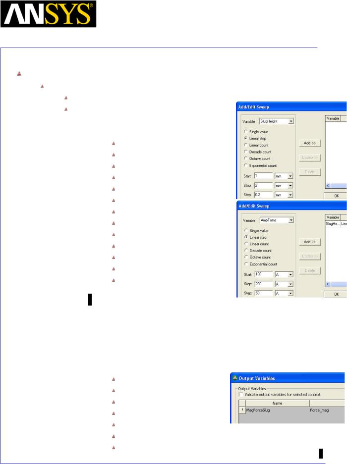
	Maxwell v15		9.4
	Basic Exercises – Parametric

Create a Parametric solution

To create Parametric Sweep

Select the menu item Maxwell 3D > Optimetrics Analysis > Add Parametric

In Setup Sweep Analysis window,

1.Select Add

2.In Add/Edit Sweep window,

Variable: SlugHeight

Linear Step:  Checked

Start: 1mm

Stop: 2mm

Step: 0.2mm

Select Add

Change Variable to AmpTurns

Linear Step:  Checked

Start: 100 A

Stop: 200 A

Step: 50 A

Select Add

Press OK

3.Change tab to Table inspect the combination of solutions that have been created. There should be 18 solutions since we defined 6 variations of SlugHeight and 3 variations of AmpTurns.

4.Select Calculations tab to set the output parameters

5.Select Setup Calculations

6.In Add/Edit Calculations window, Select Output Variables

7.In Output Variables window,

Parameter: Force1

Category: Force

Quantity: Force_mag

Select Insert Into Expression

Name: MagForceSlug

Select Add

Select Done to close window

ANSYS Maxwell 3D Field Simulator v15 User’s Guide	9.4-7

	Maxwell v15		9.4
	Basic Exercises – Parametric

8. In Add/Edit Variable window,

Parameter: Force1

Category: Output Variables

Quantity: MagForceSlug

Select Add Calculation

Select Done to close window

9. Select Options tab on Setup Sweep Analysis window

Save Fields and Mesh:  Checked

Copy geometrically equivalent meshes:  Checked 10. Click OK to close

Solve the Parametric problem

To Solve Parametric Setup

In Project manager window, expand the tree for Optimetrics

Right click on the tab Parametric Setup1 and select Analyze

Note: the solving criteria is taken from the nominal problem, Setup1 . Each parametric solution will re-mesh if the geometry has changed or the energy error criteria is not met as defined in Setup1.

ANSYS Maxwell 3D Field Simulator v15	User’s Guide	9.4-8

	Maxwell v15		9.4
	Basic Exercises – Parametric

View Analysis Results

To view the Results of Parametric Sweep

In Project manager window, expand the tree for Optimetrics

Right click on the tab Parametric Setup1 and select View Analysis Results

In Post Analysis Display window,

1. View: Select Table to view results in tabular form

Graph the Force vs. AmpTurns vs. SlugHeight

To Create a Plot

Select the menu item Maxwell 3D > Results > Create Magnetostatic Report > Rectangular Plot

In report window,

1.Parameter: Force1

2.Parametric Sweep: SlugHeight

3.X : Default

4.Y :

Category: Output Variables

Qantity: MagForceSlug

5. Select New Report

ANSYS Maxwell 3D Field Simulator v15 User’s Guide			9.4-9

	Maxwell v15		9.4
	Basic Exercises – Parametric

The Plot should appear as shown in below

Right click on the plot and select export to export the data in text file

Create a Table of SlugHeight, Force, and AmpTurns

To Create a Table

Select the menu item Maxwell 3D > Results > Create Magnetostatic Report > Data Table

In report window,

1.Parameter: Force1

2.Parametric Sweep: SlugHeight

3.X : Default

4.Y :

Category: Output Variables

Qantity: MagForceSlug

5. Select New Report

ANSYS Maxwell 3D Field Simulator v15 User’s Guide					9.4-10

	Maxwell v15		9.5
	Basic Exercises – Transient

Inductor using Transient Source

This exercise will discuss how to use transient sources as the excitation for an inductor coil.

Create Design

To Create Design

Select the menu item Project > Insert Maxwell 3D Design, or click on the icon

Change the name of the Design to BE_Trans

Set Solution Type

To set the Solution Type:

Select the menu item Maxwell 3D > Solution Type

Solution Type Window:

1.Choose Magnetic > Transient

2.Click the OK button

Create Core

Create Regular Polyhedron

Select the menu item Draw > Regular Polyhedron

1. Using the coordinate entry fields, enter the center of the base

X: 0, Y: 0, Z: 0, Press the Enter key

2. Using the coordinate entry fields, enter the radius

dX: 2, dY: 2, dZ: 0, Press the Enter key

3. Using the coordinate entry fields, enter the height

dX: 0, dY: 0, dZ:20, Press the Enter key 4. Number of Segments: 24

Change the name of the Object to Core Change the material of the object to ferrite

ANSYS Maxwell 3D Field Simulator v15 User’s Guide					9.5-1

			Maxwell v15		9.5
			Basic Exercises – Transient
		Create Coil
		Create Regular Polyhedron
		Select the menu item Draw > Regular Polyhedron
1.			Using the coordinate entry fields, enter the center of the base
			X: 0, Y: 0, Z: 0, Press the Enter key
2.			Using the coordinate entry fields, enter the radius
			dX: 3, dY: 3, dZ: 0, Press the Enter key
3.			Using the coordinate entry fields, enter the height
			dX: 0, dY: 0, dZ:20, Press the Enter key
4.			Number of Segments: 24
		Change the name of the Object to Coil
		Change the material of the object to copper
		Subtract Objects
		Press Ctrl and select the objects Coil and Core from the history tree
		Select the menu item, Modeler > Boolean > Subtract
1.			Blank Parts: Coil
2.			Tool Parts: Core
3.			Clone tool objects before operation:  Checked
4.			Click the OK button

Create CoilTerminal

To Create Coil terminal

Select the object Coil from the history tree

Select the menu item Modeler > Surface > Section

1.Section Plane: YZ

2.Press OK

Change the name of the resulting sheet to Terminal

Separate Sheets

Select the sheet Terminal from the history tree

Select the menu item Modeler > Boolean > Separate Bodies

Delete Extra Sheet

Select the sheet Terminal_Separate1 from the history tree

Select the menu item Edit > Delete

ANSYS Maxwell 3D Field Simulator v15 User’s Guide					9.5-2

	Maxwell v15		9.5
	Basic Exercises – Transient

Assign Excitation

Specify Dataset

The excitation for this problem will be a voltage source with a 1KHz triangular wave superimposed on a 50 Hz sine wave that has a 50 volt DC offset.Triangular wave will be specified through a design dataset

Select the menu item Maxwell 3D > Design Datasets

In Datasets window, select Add In Add Dataset window,

Name: DSet_A
Coordinates:
1.	X1	= 0	Y1	= 0
2.	X2	= 250e-6	Y2	= 1
3.	X3	= 750e-6	Y3	= -1
4.	X4	= 1e-3	Y4	= 0

Select OK and Done

To Assign Coil Terminal

Select the sheet Terminal from the history tree

Select the menu item Maxwell 3D > Excitations > Assign > Coil Terminal

In Current Excitation window,

1.Name: CoilTerminal1

2.Number of Conductors: 150

3. Press OK

ANSYS Maxwell 3D Field Simulator v15 User’s Guide	9.5-3

Maxwell v15

9.5

Basic Exercises – Transient

To Add Winding

Select the menu item Maxwell 3D > Excitations > Add Winding

In Winding window,

1.Name: Winding_A

2.Type: Voltage

3.Stranded:  Checked

4.Initial Current: 0 A

5.Resistance: 25 ohm

6.Inductance: 0 H

7.Voltage: 50 + 25*sin(2*PI*50*Time) + 5*pwl_periodic(DSet_A, Time)

8.Press OK

Note: The expression specified for Voltage has three different components

1.The first term is a 50 V DC offset

2.The second term is a 25 Vp-p, 50 Hz sine wave

3.The third term is a 5 Vp-p, 1 KHz triangular wave

Add Terminal to Winding

In Project manager window, expand the tree for Excitations

Right click on the tab CoilTerminal1 and select Add to Winding

In Add to Winding window,

1.Select Winding_A

2.Press OK

Note: An insulation boundary is not needed between the core and the coil because the ferrite core has a conductivity = 0.01S/m which below the default conductor/insulation threshold of 1S/m.

ANSYS Maxwell 3D Field Simulator v15 User’s Guide	9.5-4

Maxwell v15

9.5

Basic Exercises – Transient

Create Region

To Create Simulation Region

Select the menu item Draw > Region

In Region window,

1.Padding all directions similarly:  Checked

2.Padding Type: Percentage Offset

Value: 500 3. Press OK

Apply Mesh Operations

The transient solver does not use the automatic adaptive meshing process, so a manual mesh needs to be created.

To Apply Mesh Operations for Core

Select the object Core from the history tree

Select the menu item Maxwell 3D > Mesh Operations > Assign > On Selection > Length Based

In Element Length Based Refinement window,

1.Name: Length1

2.Restrict Length Of Elements:  Unchecked

3.Restrict the Number of Elements:  Checked

4.Maximum Number of Elements: 1000

5.Press OK

To Apply Mesh Operations for Coil

Select the object Coil from the history tree

Select the menu item Maxwell 3D > Mesh Operations > Assign > On

Selection > Length Based

In Element Length Based Refinement window,

1.Name: Length2

2.Restrict Length Of Elements:  Unchecked

3.Restrict the Number of Elements:  Checked

4.Maximum Number of Elements: 1000

5.Press OK

ANSYS Maxwell 3D Field Simulator v15 User’s Guide					9.5-5

	Maxwell v15		9.5
	Basic Exercises – Transient

Analysis Setup

To create an analysis setup:

Select the menu item Maxwell 3D > Analysis Setup > Add Solution Setup

Solution Setup Window: 1. General tab

Stop Time: 20 ms Time Step: 100 us

2. Click the OK button

Analyze

To run Solution

Select the menu item Maxwell 3D > Analyze All

ANSYS Maxwell 3D Field Simulator v15 User’s Guide					9.5-6

	Maxwell v15		9.5
	Basic Exercises – Transient

Plot the Voltage and Current

To Create Plots

Select the menu item Maxwell 3D > Results > Create Transient Report > Rectangular Plot

In Reports window,

1.Category: Winding

2.Quantity: Current (Winding_A)

3.Select New Report

4.Change Quantity to InputVoltage (Winding_A)

5.Select New Report

ANSYS Maxwell 3D Field Simulator v15 User’s Guide					9.5-7

	Maxwell v15		9.6
	Basic Exercises – Transient with Circuits

Inductor using Transient Source with External Circuits

This exercise will discuss how to link a transient source generated by an external circuit to an inductor coil.

Create Design

To Create Design

Select the menu item Project > Insert Maxwell 3D Design, or click on the icon

Change the name of the Design to BE_Trans_Ckt

Set Solution Type

To set the Solution Type:

Select the menu item Maxwell 3D > Solution Type

Solution Type Window:

1.Choose Magnetic > Transient

2.Click the OK button

Create Core

Create Regular Polyhedron

Select the menu item Draw > Regular Polyhedron

1. Using the coordinate entry fields, enter the center of the base

X: 0, Y: 0, Z: 0, Press the Enter key

2. Using the coordinate entry fields, enter the radius

dX: 2, dY: 2, dZ: 0, Press the Enter key

3. Using the coordinate entry fields, enter the height

dX: 0, dY: 0, dZ:20, Press the Enter key 4. Number of Segments: 24

Change the name of the Object to Core Change the material of the object to ferrite

ANSYS Maxwell 3D Field Simulator v15 User’s Guide					9.6-1

			Maxwell v15		9.6
			Basic Exercises – Transient with Circuits
		Create Coil
		Create Regular Polyhedron
		Select the menu item Draw > Regular Polyhedron
1.			Using the coordinate entry fields, enter the center of the base
			X: 0, Y: 0, Z: 0, Press the Enter key
2.			Using the coordinate entry fields, enter the radius
			dX: 3, dY: 3, dZ: 0, Press the Enter key
3.			Using the coordinate entry fields, enter the height
			dX: 0, dY: 0, dZ:20, Press the Enter key
4.			Number of Segments: 24
		Change the name of the Object to Coil
		Change the material of the object to copper
		Subtract Objects
		Press Ctrl and select the objects Coil and Core from the history tree
		Select the menu item, Modeler > Boolean > Subtract
1.			Blank Parts: Coil
2.			Tool Parts: Core
3.			Clone tool objects before operation:  Checked
4.			Click the OK button

Create CoilTerminal

To Create Coil terminal

Select the object Coil from the history tree

Select the menu item Modeler > Surface > Section

1.Section Plane: YZ

2.Press OK

Change the name of the resulting sheet to Terminal

Separate Sheets

Select the sheet Terminal from the history tree

Select the menu item Modeler > Boolean > Separate Bodies

Delete Extra Sheet

Select the sheet Terminal_Separate1 from the history tree

Select the menu item Edit > Delete

ANSYS Maxwell 3D Field Simulator v15 User’s Guide					9.6-2

	Maxwell v15		9.6
	Basic Exercises – Transient with Circuits

Assign Excitation

To Assign Coil Terminal

Select the sheet Terminal from the history tree

Select the menu item Maxwell 3D > Excitations > Assign > Coil Terminal

In Current Excitation window,

1.Name: CoilTerminal1

2.Number of Conductors: 150

3.Press OK

To Add Winding

Select the menu item Maxwell 3D > Excitations > Add Winding

In Winding window,

1.Name: Winding_A

2.Type: External

3.Stranded:  Checked

4.Initial Current: 0 A

5.Press OK

Add Terminal to Winding

In Project manager window, expand the tree for Excitations

Right click on the tab CoilTerminal1 and select Add to Winding

In Add to Winding window,

1.Select Winding_A

2.Press OK

Note: An insulation boundary is not needed between the core and the coil because the ferrite core has a conductivity = 0.01S/m which below the default conductor/insulation threshold of 1S/m.

ANSYS Maxwell 3D Field Simulator v15 User’s Guide							9.6-3

	Maxwell v15		9.6
	Basic Exercises – Transient with Circuits

Create External Circuit

To Launch Maxwell Circuit Editor

To access Maxwell Circuit Editor, click the Microsoft Start button, select Programs > Ansoft > Maxwell 15> Maxwell Circuit Editor

To Add Components

Change the tab in Project Manager window to Components

In Project Manager window, expand the tree for Maxwell Circuit Elements > Dedicated Elements . Select the element Winding from the tree, drag and drop it on the worksheet

Select the winding added in worksheet and go to the properties window, 1. Change the name of the winding to Winding_A

Note: This name has to be exactly the same as used in Maxwell in Maxwell 3D > Excitations > Add Winding

In Project Manager window, select Sources > VSin from the tree, drag and drop it on the worksheet. Select the source added in worksheet and go to the properties window,

1.Change the value of Va to 100 V

2.Change the value of VFreq to 50 Hz

Add another source VSin and change its properties as below

1.Change the value of Va to 10 V

2.Change the value of VFreq to 1000 Hz

In Project Manager window, select Passive Elements > Res , drag and drop it on the worksheet. Select the resistor added in worksheet and go to the properties window,

1. Change the value of R to 25 ohm

ANSYS Maxwell 3D Field Simulator v15 User’s Guide	9.6-4

	Maxwell v15		9.6
	Basic Exercises – Transient with Circuits

In Project Manager window, select Probes > Voltmeter, drag and drop it on the worksheet

Select the menu item Draw > Wire to draw wires Select the menu item Draw > Ground to add ground Build the circuit as shown in below image

Note: Same name used:

Winding_A

To Export Circuit

Select the menu item Maxwell Circuit > Export Netlist

1. Save the file with the name BE_Circuit.sph To Save File

Select the menu item File > Save

1. Save the file with the name BE_Circuit.amcp

Link the circuit file to the Maxwell project

To Import circuit in Maxwell

Return to Maxwell window

In Maxwell, Select the menu item Maxwell 3D > Excitations > External Circuit > Edit External Circuit

In Edit External Circuit window,

1.Select Import Circuit

2.Browse to the file BE_Circuit.sph and Open it

3.Press OK

ANSYS Maxwell 3D Field Simulator v15 User’s Guide					9.6-5

Maxwell v15

9.6

Basic Exercises – Transient with Circuits

Create Region

To Create Simulation Region

Select the menu item Draw > Region

In Region window,

1.Padding all directions similarly:  Checked

2.Padding Type: Percentage Offset

Value: 500

3. Press OK

Apply MeshOperations

The transient solver does not use the automatic adaptive meshing process, so a manual mesh needs to be created.

To Apply Mesh Operations for Core

Select the object Core from the history tree

Select the menu item Maxwell 3D > Mesh Operations > Assign > On Selection > Length Based

In Element Length Based Refinement window,

1.Name: Length1

2.Restrict Length Of Elements:  Unchecked

3.Restrict the Number of Elements:  Checked

4.Maximum Number of Elements: 1000

5.Press OK

To Apply Mesh Operations for Coil

Select the object Coil from the history tree

Select the menu item Maxwell 3D > Mesh Operations > Assign > On

Selection > Length Based

In Element Length Based Refinement window,

1.Name: Length2

2.Restrict Length Of Elements:  Unchecked

3.Restrict the Number of Elements:  Checked

4.Maximum Number of Elements: 1000

5.Press OK

ANSYS Maxwell 3D Field Simulator v15 User’s Guide					9.6-6

	Maxwell v15		9.6
	Basic Exercises – Transient with Circuits

Analysis Setup

To create an analysis setup:

Select the menu item Maxwell 3D > Analysis Setup > Add Solution Setup

Solution Setup Window: 1. General tab

Stop Time: 20 ms Time Step: 100 us

2. Click the OK button

Analyze

To run Solution

Select the menu item Maxwell 3D > Analyze All

ANSYS Maxwell 3D Field Simulator v15 User’s Guide					9.6-7

	Maxwell v15		9.6
	Basic Exercises – Transient with Circuits

Plot the Voltage and Current

To Create Plots

Select the menu item Maxwell 3D > Results > Create Transient Report > Rectangular Plot

In Reports window,

1.Category: Winding

2.Quantity: Current (Winding_A)

3.Select New Report

4.Change Category to NodeVoltage

5.Quantity: NodeVoltage

6.Select New Report

ANSYS Maxwell 3D Field Simulator v15 User’s Guide					9.6-8

	Maxwell v15		9.7
	Basic Exercises – Post Processing

Post Processing in Maxwell 3D

This exercise will discuss how to use the Maxwell 3D Post Processor. Field plots and calculator operations will demonstrated on an Eddy Current project. The following tasks will be performed:

Plot the mesh on the core and coil

Plot of MagB on a plane

Plot of B_vector on a plane

Plot of MagH along a line

Create a table of MagH along a line

Calculate average MagB in an object

Verify DivB = 0

Calculate flux flowing through the top surface of the core

Calculate loss in the conductor

Calculate net and total current flowing in the conductor Export field results to a file.

Create Design

To Create Design

Select the menu item Project > Insert Maxwell 3D Design, or click on the icon

Change the name of the Design to Post_Exercise

Set Solution Type

To set the Solution Type:

Select the menu item Maxwell 3D > Solution Type

Solution Type Window:

1.Choose Magnetic > Eddy Current

2.Click the OK button

ANSYS Maxwell 3D Field Simulator v15 User’s Guide							9.7-1

					Maxwell v15		9.7
					Basic Exercises – Post Processing
		Create Core
		Create Regular Polyhedron
				Select the menu item Draw > Regular Polyhedron
1.					Using the coordinate entry fields, enter the center of the base
					X: 0, Y: 0, Z:-10, Press the Enter key
2.					Using the coordinate entry fields, enter the radius
					dX: 0, dY: 5, dZ: 0, Press the Enter key
3.					Using the coordinate entry fields, enter the height
					dX: 0, dY: 0, dZ:20, Press the Enter key
4.					Number of Segments: 24
				Change the name of the Object to Core and material to iron
		Create		Coil
		Create Regular Polyhedron
				Select the menu item Draw > Regular Polyhedron
1.					Using the coordinate entry fields, enter the center of the base
					X: 0, Y: 0, Z: 0, Press the Enter key
2.					Using the coordinate entry fields, enter the radius
					dX: 10, dY: 0, dZ: 0, Press the Enter key
3.					Using the coordinate entry fields, enter the height
					dX: 0, dY: 0, dZ:2, Press the Enter key
4.					Number of Segments: 24
				Change the name of the Object to Coil and material to copper
		Create Hole
				Select the menu item Draw > Regular Polyhedron
1.					Using the coordinate entry fields, enter the center of the base
					X: 0, Y: 0, Z: 0, Press the Enter key
2.					Using the coordinate entry fields, enter the radius
					dX: 8, dY: 0, dZ: 0, Press the Enter key
3.					Using the coordinate entry fields, enter the height
					dX: 0, dY: 0, dZ:2, Press the Enter key
4.					Number of Segments: 24

Change the name of the Object to Hole

ANSYS Maxwell 3D Field Simulator v15 User’s Guide			9.7-2

Maxwell v15

9.7

Basic Exercises – Post Processing

Subtract Objects

Press Ctrl and select the objects Coil and Hole from the history tree

Select the menu item, Modeler > Boolean > Subtract

1.Blank Parts: Coil

2.Tool Parts: Hole

3.Click the OK button

Create Coil Terminal

To Create Coil terminal

Select the object Coil from the history tree

Select the menu item Modeler > Surface > Section

1.Section Plane: YZ

2.Press OK

Change the name of the resulting sheet to Terminal

Separate Sheets

Select the sheet Terminal from the history tree

Select the menu item Modeler > Boolean > Separate Bodies

Delete Extra Sheet

Select the sheet Terminal_Separate1 from the history tree

Select the menu item Edit > Delete

Create a line for plotting of the fields

To Create a Line

Select the menu item Draw > Line

1. Using the coordinate entry fields, enter the first vertex

X: 0, Y: 0, Z: 0, Press the Enter key

2. Using the coordinate entry fields, enter the second vertex X: 0, Y: 0, Z: 20, Press the Enter key

3. Press Enter to exit line creation

ANSYS Maxwell	3D Field Simulator v15 User’s Guide					9.7-3

Maxwell v15

9.7

Basic Exercises – Post Processing

Assign Excitation

To Assign Excitation

Select the sheet Terminal from the history tree

Select the menu item Maxwell 3D > Excitations > Assign > Current

In Current Excitation window,

1.Name: Current1

2.Value: 100 A

3.Phase: 0

4.Type: Solid (eddy effects can only be determined in solid sources)

5.Direction: Point out of terminal

6.Press OK

Create Region

To Create Simulation Region

Select the menu item Draw > Region

In Region window,

1.Padding all directions similarly:  Checked

2.Padding Type: Percentage Offset

Value: 100

3. Press OK

Set Eddy Effect

To Set Eddy Calculations

Select the menu item Maxwell 3D > Excitations > Set Eddy Effect

In Set Eddy Effect window, 1. Core

Eddy Effects:  Unchecked 2. Press OK

ANSYS Maxwell 3D Field Simulator v15 User’s Guide			9.7-4

			Maxwell v15				9.7
					Basic Exercises – Post Processing
		Setup the Impedance Calculation
		To Setup Impedance Calculations
		Select the menu item Maxwell 3D > Parameters > Assign > Matrix
		In Matrix window,
1.			Current1:
					Include:  Checked
2.			Press OK

Apply Mesh Operations

In order to create a fine initial mesh, several mesh operation will be performed.

To Apply Mesh Operations for Core

Select the object Core from the history tree

Select the menu item Maxwell 3D > Mesh Operations > Assign > On Selection > Length Based

In Element Length Based Refinement window,

1.Name: Length1

2.Restrict Length Of Elements:  Unchecked

3.Restrict the Number of Elements:  Checked

4.Maximum Number of Elements: 5000

5.Press OK

To Apply Mesh Operations for Coil

Select the object Coil from the history tree

Select the menu item Maxwell 3D > Mesh Operations > Assign > On

Selection > Length Based

In Element Length Based Refinement window,

1.Name: Length2

2.Restrict Length Of Elements:  Unchecked

3.Restrict the Number of Elements:  Checked

4.Maximum Number of Elements: 5000

5.Press OK

ANSYS Maxwell 3D Field Simulator v15 User’s Guide	9.7-5

	Maxwell v15		9.7
	Basic Exercises – Post Processing

Analysis Setup

To create an analysis setup:

Select the menu item Maxwell 3D > Analysis Setup > Add Solution Setup

Solution Setup Window: 1. Solver tab

Adaptive Frequency: 100 kHz 2. Click the OK button

Validation Check

To Check the Validation of Case

Select the menu item Maxwell 3D > Validation Check

Analyze

To run Solution

Select the menu item Maxwell 3D > Analyze All

ANSYS Maxwell 3D Field Simulator v15 User’s Guide					9.7-6

	Maxwell v15		9.7
	Basic Exercises – Post Processing

Solution Data

To view the Solution Data:

Select the menu item Maxwell 3D > Results > Solution Data

To view the Profile:

1. Click the Profile Tab. To view the Convergence:

1. Click the Convergence Tab

Note: The default view is for convergence is Table. Select the Plot radio button to view a graphical representations of the convergence data.

To View Mesh information

1. Click Mesh Statistics Tab

ANSYS Maxwell 3D Field Simulator v15	User’s Guide			9.7-7

	Maxwell v15		9.7
	Basic Exercises – Post Processing

To View Impedance values

1.Click Matrix tab

2.Set Type to Re(Z), Im(Z)

Note: the imaginary term of the matrix includes both the inductive and capacitive reactance are reported in Ohms.

3. Change Type to R,L

Note: Imaginary term of the matrix includes only the inductance and is reported in Ohms and Henries

Plot Mesh

To Plot Mesh on Core and Coil

Press Ctrl and select the objects Core and Coil

Select the menu item Maxwell 3D > Fields > Plot Mesh

In Create Mesh Plot window, 1. Press Done

ANSYS Maxwell 3D Field Simulator v15 User’s Guide							9.7-8

Maxwell v15

9.7

Basic Exercises – Post Processing

Plot Mag_B on Core

To Plot Mag_B

Select the object Core from the history tree

Select the menu item Maxwell 3D > Fields > Fields > B > Mag_B

In Create Field Plot window,

1.Plot on surface only:  Checked

2.Press Done

Plot Vector_B on YZ Plane

To Plot Vector_B on a Plane

Expand the tree for Planes in History tree and select the pane Global:YZ

Select the menu item Maxwell 3D > Fields > Fields > B > Vector_B

In Create Field Plot window 1. Press Done

To Modify Attributes

Double click on the legend to change plot properties

In the window

1. Marker/Arrow tab

Arrow Options

1. Size: Set to appropriate value

2. Plots tab

Vector Plot

1.Spacing: Minimum

2.Min: 1

3.Max: 3

3.Press Apply and Close

ANSYS	Maxwell 3D Field Simulator v15 User’s Guide					9.7-9

	Maxwell v15		9.7
	Basic Exercises – Post Processing

Plot Mag_H along a Line

To Plot Mag_H

Select the menu item Maxwell 3D > Results > Create Field Reports > Rectangular Plot

In Report window.

1.Geometry: Polyline1

2.X : Default

3.Category: Calculator Expressions

4.Quantity: Mag_H

5.Select New Report

Table of Mag_H along a Line

Select the menu item Maxwell 3D > Results > Create Field Reports > Data Table

In Report window.

1.Geometry: Polyline1

2.X : Default

3.Category: Calculator Expressions

4.Quantity: Mag_H

5.Select New Report

ANSYS Maxwell 3D Field Simulator v15 User’s Guide							9.7-10

Maxwell v15

9.7

Basic Exercises – Post Processing

Calculate Average Mag_B in an Object

To Calculate Mag_B Over a Volume

Select the menu item Maxwell 3D > Fields > Calculator

1.Select Input > Quantity > B

2.Select General > Complex > Real

3.Select Vector > Mag

4.Select Input > Geometry

Volume:  Checked

Select Core from the list

Press OK

5.Select Scalar > Integrate

6.Select Input > Number

Scalar:  Checked

Value: 1

Press OK

7. Select Input > Geometry

Volume:  Checked

Select Core from the list Press OK

8.Select Scalar > Integrate

9.Select General > / (Divide)

10.Select Output > Eval

The average value of flux density calculated is around 0.036 Tesla

ANSYS Maxwell 3D Field Simulator v15 User’s Guide			9.7-11

Maxwell v15

9.7

Basic Exercises – Post Processing

Calculate DivB = 0

To Calculate DivB

Select the menu item Maxwell 3D > Fields > Calculator

1.Select Input > Quantity > B

2.Select General > Complex > Real

3.Select Vector > Divg

4.Select Input > Geometry

Volume:  Checked

Select Core from the list

Press OK

5.Select Scalar > Integrate

6.Select Output > Eval

The divergence of B is approximately zero

Calculate flux flowing out of the top surface of the core

To Calculate flux

Select the menu Edit > Select > Faces or press F from keyboard

Select the menu item Modeler > List > Create > Face List

Select the top face of the Core as shown in below image Select the menu item Maxwell 3D > Fields > Calculator

1.Select Input > Quantity > B

2.Select General > Complex > Real

3.Select Input > Geometry

Surface:  Checked

Select Facelist1 from the list

Press OK

4.Select Vector > Normal

5.Select Scalar > Integrate

6.Select Output > Eval

The net flux flowing out of the core is approximately (1.1 e-6 Webers)

ANSYS Maxwell 3D Field Simulator v15 User’s Guide					9.7-12

	Maxwell v15		9.7
	Basic Exercises – Post Processing

Calculate loss in a conductor

To calculate losses in Coil

1.Select Input > Quantity > OhmicLoss

2.Select Input > Geometry

Volume:  Checked

Select Coil from the list

Press OK

3.Select Scalar > Integrate

4.Select Output > Eval

The ohmic loss in the coil at 100 kHz is approximately 2.66 Watts.

Calculate the current flowing in a conductor

To Calculate Net Current in Coil

1.Select Input > Quantity > J

2.Select General > Complex > Real

3.Select Input > Geometry

Surface:  Checked

Select Terminal from the list

Press OK

4.Select Vector > Normal

5.Select Scalar > Integrate

6.Select Output > Eval

The net current in the coil is equal to the source amp-turns = +/- 100

Calculate Total Current including Eddy Component

1.Select Input > Quantity > J

2.Select General > Complex > CmplxMag

3.Select Input > Geometry

Surface:  Checked

Select Terminal from the list

Press OK

4.Select Vector > Normal

5.Select Scalar > Integrate

6.Select Output > Eval

Calculated value of current comes out to be around 120 A

ANSYS Maxwell 3D Field Simulator v15 User’s Guide	9.7-13

	Maxwell v15		9.7
	Basic Exercises – Post Processing

Export field results to a file

In order to use the field results in another software program, you can export the fields on a uniform 3-dimensional grid.

To Export Results

1.Select Input > Quantity > H

2.Select Output > Export

3.In Export Solution window,

Output file name: H_Vector

Calculate grid points:  Checked

Minimum: (0, 0,0)

Maximum: (5, 5, 5)

Spacing: (1, 1, 1)

Minimum: The minimum coordinates of the grid, and unit of measure

Maximum: The maximum coordinates of the grid, and unit of measure

Spacing: The distance between grid points, and unit of measure

ANSYS Maxwell 3D Field Simulator v15 User’s Guide					9.7-14

	Maxwell v15		9.8
	Basic Exercises – Optimetrics

Puck Magnet Attractor

This example describes how to create and optimize a puck magnet producing an optimal force on a steel plate using the 3D Magnetostatic solver and Optimetrics in the ANSYS Maxwell 3D Design Environment.

The optimization obtains the desired force by varying the air gap between the plate and the puck using a local variable.

Create Design

To Create Design

Select the menu item Project > Insert Maxwell 3D Design, or click on the icon

Change the name of the Design to Puck_Attractor

Set Solution Type

To set the Solution Type:

Select the menu item Maxwell 3D > Solution Type

Solution Type Window:

1.Choose Magnetic > Magnetostatic

2.Click the OK button

ANSYS Maxwell	3D Field Simulator v15 User’s Guide					9.8-1

Maxwell v15

9.8

Basic Exercises – Optimetrics

Create Steel Plate

To Create Steel Plate

Select the menu item Draw > Box

1. Using the coordinate entry fields, enter the position of box

X: -10, Y: -10, Z: 0, Press the Enter key

2. Using the coordinate entry fields, enter the opposite corner

dX: 20, dY: 20, dZ: -1, Press the Enter key

Change the name of the Object to Plate Change the material of the Object to steel_1008

Create Puck

To Create Puck

Select the menu item Draw > Regular Polyhedron

1. Using the coordinate entry fields, enter the center of the base

X: 0, Y: 0, Z: 2, Press the Enter key

2. Using the coordinate entry fields, enter the radius

dX: 2, dY: 2, dZ: 0, Press the Enter key

3. Using the coordinate entry fields, enter the height

dX: 0, dY: 0, dZ:2, Press the Enter key 4. Number of Segments: 12

Change the name of the Object to Puck Change the material of the Object to NdFe30

ANSYS Maxwell 3D Field Simulator v15 User’s Guide					9.8-2

Maxwell v15

9.8

Basic Exercises – Optimetrics

Create Parameter for Puck Motion

To Create Puck Motion

Select the Object Puck from the history tree

Select the menu item Edit > Arrange > Move

1.Using the coordinate entry fields, enter the reference point of move vector

X: 0, Y: 0, Z: 0, Press the Enter key

2.Using the coordinate entry fields, enter the target point of move vector

dX: 0, dY: 0, dZ: 0, Press the Enter key

To Parameterize Puck Motion

Expand the history tree for the Object Puck

Double click on the command Move from the tree

In Properties window,

1.Move Vector: Specify as 0, 0, move

2.In Add variable window,

Unit Type: Length

Unit: mm

Value: 0

Press OK

3. Press OK to close Properties window

ANSYS Maxwell 3D Field Simulator v15 User’s Guide					9.8-3

	Maxwell v15		9.8
	Basic Exercises – Optimetrics

Create Relative Coordinate System

Note: In Maxwell, all magnetic materials are magnetized in X direction. In this step, we will change the direction of magnetization for puck by creating relative coordinate system.

To Create Relative Coordinate System

Select the menu item Modeler > Coordinate System > Create > Relative CS > Rotated

1. Using the coordinate entry fields, enter the X axis

X: 0, Y: 0, Z: 1, Press the Enter key

2. Using the coordinate entry fields, enter a point on XY Plane

dX: 0, dY: 1, dZ: 0, Press the Enter key

To Assign Coordinate System to Puck

Select the object Puck from the history tree and goto the properties window Change the Orientation of the object to RelativeCS1

Assign Parameters Force

To Assign Force Parameter

Select the object Plate from the history tree

Select the menu item Maxwell 3D > Parameters > Assign > Force

In Force Setup window,

1.Name: Force

2.Type: Virtual

3.Press OK

ANSYS Maxwell 3D Field Simulator v15 User’s Guide					9.8-4

Maxwell v15

9.8

Basic Exercises – Optimetrics

Create Region

To Change Work Coordinate System

Select the menu item Modeler > Coordinate System . Set Work CS

1.Select the coordinate System Global from the list

2.Press Select

To Create Simulation Region

Select the menu item Draw > Region

In Region window,

1.Padding individual directions:  Checked

2.Value:

+/- X = 100

+/- Y = 100 +/- Z = 500

3. Press OK

Analysis Setup

To create an analysis setup:

Select the menu item Maxwell 3D > Analysis Setup > Add Solution Setup

Solution Setup Window: 1. General tab

Percentage Error: 2 2. Convergence tab

Refinement Per Pass: 50%

Validation Check

To Check the Validation of Case

Select the menu item Maxwell 3D > Validation Check

Note: To view any errors or warning messages, use the Message Manager.

Analyze

To run Solution

Select the menu item Maxwell 3D > Analyze All

ANSYS Maxwell 3D Field Simulator v15 User’s Guide	9.8-5

	Maxwell v15		9.8
	Basic Exercises – Optimetrics

Solution Data

To view the Solution Data:

Select the menu item Maxwell 3D > Results > Solution Data

To view the Profile:

1. Click the Profile Tab. To view the Convergence:

1. Click the Convergence Tab

Note: The default view is for convergence is Table. Select the Plot radio button to view a graphical representations of the convergence data.

To View Mesh information

1. Click Mesh Statistics Tab

To View Force values

1. Click Force tab

ANSYS Maxwell 3D Field Simulator v15	User’s Guide			9.8-6

	Maxwell v15		9.8
	Basic Exercises – Optimetrics

Optimetrics Setup and Solution

It is possible to optimize position in order to obtain the specified force. For this optimization, the position will be varied to obtain a desired force of 0.25N.

Specify Parametric Variables

Select the menu item Maxwell 3D > Design properties

In Properties window,

1.Optimization:  Checked

2.move:

Include:  Checked

Min : 0 mm

Max : 1 mm 3. Press OK

Setup an Optimization Analysis

Select the menu item Maxwell 3D > Optimetrics Analysis > Add

Optimization

In Setup Optimization window,

1.Optimizer: Sequential Nonlinear Programming

2.Max. No. of Iterations: 10

3.Select Setup Calculations

4.In Add/Edit calculations window, select Output Variables

5.In Output variables window,

Name: target

Expression: 0.25

Select Add

Without closing window, set name to cost1

Set Parameter to Force1

Expression: (target – Force_z)^2

Press Done

ANSYS Maxwell 3D Field Simulator v15 User’s Guide			9.8-7

Maxwell v15

9.8

Basic Exercises – Optimetrics

6. In Add/Edit Calculations window,

Parameter : Force1

Category: Output Variables

Quantity: cost1

Select Add Calculation Press Done

7.Parameter cost1 will be added to Setup Optimization window.

8.Set Condition for cost1 to Minimize

9.Change the tab to Variables

10.For the variable move

Starting value: 0.5mm

Min: 0 mm

Max: 1 mm

Min Focus: 0.1 mm

Max Focus: 0.9 mm

Press OK

ANSYS Maxwell 3D Field Simulator v15 User’s Guide			9.8-8

	Maxwell v15		9.8
	Basic Exercises – Optimetrics

Solve Optimization Analysis

To Solve Optimization Analysis

Select the menu item Maxwell 3D > Analyze All

View Optimetrics Results

To View Results

Select the menu item Maxwell 3D > Optimetrics Analysis > Optimetrics Results

In Post Analysis Display window, 1. Log Scale:  Checked

Plot Display should look as below

Change View to Table to see actual values

Press Close

ANSYS Maxwell 3D Field Simulator v15 User’s Guide	9.8-9

	Maxwell v15		9.8
	Basic Exercises – Optimetrics

Create Plot of Cost vs Move

To Create Report

Select menu item Maxwell 3D > Results > Create Magnetostatic Report > Rectangular Plot

In Report window,

1.Parameter: Force1

2.X : Default

3.Category: Output Variables

4.Quantity: cost1

5.Function: <none>

6.Select New Report

To Modify Plot Attributes

Double click on Y axis of plot

In Properties window,

1. Scaling tab

Axis Scaling: Log

Pres OK

From the plot, it can be seen that minimum value of cost is obtained at around 445 um

ANSYS Maxwell 3D Field Simulator v15 User’s Guide			9.8-10

	Maxwell v15		9.9
	Basic Exercises – Meshing Operations

Introduction on Meshing Operations

This note introduces the different mesh operations that Maxwell offers. Mesh operation are used either to cut the number of adaptive passes or to optimize the mesh details on complicated objects. We will illustrate the meshing operations using an SRM core.

Create Design

To Create Design

Select the menu item Project > Insert Maxwell 3D Design, or click on the

icon

Create Core

To Create Core

Select the menu item Draw> User Define Primitive > SysLib > RMxprt > SRMcore

In User Defined Primitive Operation window, 1. Press OK to accept default settings

Change the name of the Object to Core

Analysis Setup

To Create Analysis Setup

Select the menu item Maxwell 3D > Analysis Setup > Add Solution Setup

In Solve Setup window,

1. Press OK to accept default settings

Save File

To Save File

Select the menu item File > Save As

1. Save the file with name Ex_9_9_BasicMeshing.mxwl

ANSYS Maxwell 3D Field Simulator v15 User’s Guide					9.9-1

	Maxwell v15		9.9
	Basic Exercises – Meshing Operations

Generate Initial Mesh

To Create Initial Mesh

Select the menu item Maxwell 3D > Analysis Setup > Apply Mesh

Operations

Plot Mesh

To Plot Mesh on the Object

Select the Object Core from the history tree

Select the menu item Maxwell 3D > Fields > Plot Mesh

In Create Mesh plot window, 1. Press Done

Note : This is initial mesh created by Maxwell. Apart from transient solver, for all other solvers this mesh will be refined for each pass in order to increase accuracy of solution. For Transient solutions, mesh refinement is not done. So it is required to apply appropriate mesh sizes which will be discussed in next few slides.

Mesh Statistics

To View Statistics of Mesh

Select the menu item Maxwell 3D > Results > Solution Data

In Solutions window,

1. Select the tab Mesh Statistics

ANSYS Maxwell 3D Field Simulator v15 User’s Guide			9.9-2

	Maxwell v15		9.9
	Basic Exercises – Meshing Operations

Mesh Operations

Maxwell3D has number of meshing operations in order to construct a better initial mesh for pass one. These mesh operations enable you to add elements in a volume, on a surface. It is also possible to monitor the discretization of true surfaces.

Note that when assigning a mesh operation, the mesh process will do its best to cope with the specified operations. Automatic meshing is a complex operation, so other constraints are to be taken into account. As a result, sometimes, the obtained mesh is not quite exactly what has been entered because internal constraints (seeding, facetting, ..) have imposed a different mesh topology. For instance, it will be difficult for the meshing engine to put 100,000 elements on the top face of a cylinder if the rest of the cylinder has a very coarse mesh.

For selected objects, five different type of mesh operations can be applied

First two operations are used to add elements either on the surface or in the volume of the objects

The last three meshing operations will monitor the way the meshing will handle the geometry of the object.

ANSYS Maxwell 3D Field Simulator v15 User’s Guide							9.9-3

	Maxwell v15		9.9
	Basic Exercises – Meshing Operations

Mesh operation: Add Elements in the Object

We can add more elements in any object to obtain a better mesh density right away.

To Apply Mesh operations in an object

Select the object Core from the history tree

Select the menu item Maxwell 3D > Mesh Operations > Assign > Inside Selection > Length Based

Mesh operations can be assigned based on either Maximum Length of Elements or Maximum Number of elements in an object.

When you enter both a number of elements and you restrict the maximum length of elements, Maxwell will stop when the first constraint is attained. In this particular case, entering only a maximum length of 10mm produces about 20,000 elements. Therefore, having both 10mm and 2,000 elements lead to have only 2,000 elements added.

ANSYS Maxwell 3D Field Simulator v15 User’s Guide	9.9-4

	Maxwell v15		9.9
	Basic Exercises – Meshing Operations

Mesh operation: Add Elements on a Surface

To Apply Mesh Operations on a Surface

Delete already applied mesh operations

Select the menu item Maxwell 3D > Analysis Setup > Revert to Initial Mesh

Select the menu item Edit > Select > Faces to change selection filter to faces

Select the face of the object as shown in the image

Select the menu item Maxwell 3D > Mesh Operations > Assign > On Selection > Length Based

Set Maximum Number of Elements to 2000

Select the menu item Maxwell 3D > Analysis Setup > Apply Mesh Operations

The resulting mesh takes into account the operation by adding elements on the surface without affecting the other parts of the object.

ANSYS Maxwell 3D Field Simulator v15 User’s Guide					9.9-5

	Maxwell v15		9.9
	Basic Exercises – Meshing Operations

Mesh operation: Skin Depth Mesh

This mesh operation has to be used with great caution. The goal is to impose to Maxwell to mesh in the skin depth with a given number of layers and a given mesh density. This can be used in the case where the skin depth is much smaller than the dimensions of the object and therefore there is a risk that the adaptive meshing won’t capture the eddy current in the early adaptive passes.

The major consequence of the mesh operation is that the adaptive meshing process does not have the full freedom when refining the mesh. Usually, it is preferred to use phantom objects or shells to take into account skin depth.

Mesh operation: Surface Approximation

This mesh operations control the way Maxwell handle true surfaces

When an object’s surface is non-planar, the faceted triangle faces lie a small distance from the object’s true surface. This distance is called the surface deviation, and it is measured in the model’s units. The surface deviation is greater near the triangle centers and less near the triangle vertices.

The normal of a curved surface is different depending on its location, but it is constant for each triangle. (In this context, “normal” is defined as a line perpendicular to the surface.) The angular difference between the normal of the curved surface and the corresponding mesh surface is called the normal deviation and is measured in degrees (15deg is the default).

To Apply Surface Approximation

Delete already applied mesh operations

Select the menu item Maxwell 3D > Analysis Setup > Revert to Initial Mesh

Select the Object Core from the history tree

Select the menu item Maxwell 3D > Mesh Operations > Assign > Surface Approximation

ANSYS	Maxwell 3D Field Simulator v15 User’s Guide					9.9-6

			Maxwell v15			9.9
			Basic Exercises – Meshing Operations

Maximum surface deviation corresponds to the distance d above Normal Surface Normal Deviation corresponds to the angle θ

In most of the cases initial mesh is created using Tau Mesher. Using Normal or High option in Surface Approximation window, we can set tolerance in capturing small features. Using High option will help in creating better mesh on small details with expense of mesh count.

In Surface Approximation window,

1.Set Maximum Aspect Ratio value to 2

2.Generate the mesh with these parameters

3.Maxwell will make sure that the elements are not too flat

ANSYS Maxwell 3D Field Simulator v15 User’s Guide					9.9-7

	Maxwell v15		9.9
	Basic Exercises – Meshing Operations

4.Edit mesh parameters and set the value of Maximum Normal Deviation angle to 5 degrees. Set all other values to default and apply mesh operations

5.Putting 5 produces 3 times more elements to discretize a curved surface

6.

7.

Set the value of maximum surface deviation length to 0.05 leaving all other values to default. This will ensure that the distance between curve lines and element edges won’t be more than 0.05mm.

The mesh operation is used when dealing with objects that have ‘small’ true surfaces (fillet, some details) and ‘large’ true surfaces.

ANSYS Maxwell 3D Field Simulator v15 User’s Guide			9.9-8

	Maxwell v15		9.9
	Basic Exercises – Meshing Operations

Mesh Operation: Model Resolution

To Set Model Resolution

Delete the previous mesh operation

Select the object Core from the history tree

Select the menu item Maxwell 3D > Mesh Operations > Assign > Model Resolution

In Model Resolution mesh Operation window,

1.Set the tab to Use Model Resolution Length

2.Set the Length value to 1mm

3.Press OK

This operation is meant to disfeature an object. By putting 1mm, Maxwell will disregard any detail below 1mm. This can be useful when dealing with imported geometries where some details, inconstancies remain. This operation is seldom used. For this piece, the result is not spectacular at all.

ANSYS Maxwell 3D Field Simulator v15 User’s Guide					9.9-9

	Maxwell v15		9.9
	Basic Exercises – Meshing Operations

Mesh Operation: Cylindrical Gap Treatment

These mesh operations are generally used to resolve narrow gaps in motor geometries . There are very small gaps between stator and rotor. The Band region created between them which needs to have fine mesh resolution between band region and stator or rotor. In such cases it is helpful to use this mesh operation on Band region.

Create Band Region

Select the menu item Draw > Cylinder

1. Using the coordinate entry fields, enter the center of the base

X: 0, Y: 0, Z: -60, Press the Enter key

2. Using the coordinate entry fields, enter the radius

dX: 51, dY: 0, dZ: 0, Press the Enter key 3. Using the coordinate entry fields, enter the height

dX: 0, dY: 0, dZ:120, Press the Enter key

Change the name of the object to Band

Assign Mesh operation

Select the object Band from the history tree

Select the menu item Maxwell 3D > Mesh Operations > Assign > Cylindrical Gap Treatment

Apply mesh operations

The refinement will be done in the region of small gap in order to capture the thin region.

ANSYS Maxwell 3D Field Simulator v15 User’s Guide					9.9-10

Maxwell v15

9.10

Basic Exercises – Scripting

Scripting the Creation of a Model Object

This exercise will discuss how to record, modify and run a script for automating the generation of a cylinder. The following tasks will be performed:

Record a script in which a cylinder is created.

Modify the script to change the cylinder’s radius and height. Run the modified script.

Create Design

To Create Design

Select the menu item Project > Insert Maxwell 3D Design, or click on the

icon

Save File

To Save File

Select the menu item File > Save As

1. Save the file with name Ex_9_10_BasicScripting.mxwl

ANSYS Maxwell 3D Field Simulator v15 User’s Guide					9.10-1

Maxwell v15

9.10

Basic Exercises – Scripting

Start Recording the Script

To Record a Script

Select the menu item Tools > Record Script to File

Save the file with the name Ex_9_10_BasicScripting.vbs

Create Cylinder

To Create Cylinder

Select the menu item Draw > Cylinder

1. Using the coordinate entry fields, enter the center of the base

X: 0, Y: 0, Z: 0, Press the Enter key

2. Using the coordinate entry fields, enter the radius

dX: 1, dY: 0, dZ: 0, Press the Enter key

3. Using the coordinate entry fields, enter the height dX: 0, dY: 0, dZ:10, Press the Enter key

Stop Script Recording

To Stop Recording a Script

Select the menu item Tools > Stop Script Recording

DeleteCylinder

To Delete Cylinder

Select the menu item Edit > Select All

Select the menu item Edit > Delete

Run Script to Recreate Cylinder

To Run Script

Select the menu item Tools > Run Script

Locate the file Ex_9_10_BasicScripting.vbs and Open it

If successful, the original cylinder, Cylinder1, should be back.

We can now explore the contents of the script file.

ANSYS Maxwell 3D Field Simulator v15 User’s Guide					9.10-2

Maxwell v15

9.10

Basic Exercises – Scripting

Open Script for Editing

To View Script

Open the script file using Textpad or Wordpad

Script File Contents

Definition of environment variables.

Dim is the generic visual basic variable type. ' ----------------------------------------------

' Script Recorded by Ansoft Maxwell Version 15.0.0 ' 3:52:27 PM Dec 14, 2011

' ----------------------------------------------

Dim oAnsoftApp

Dim oDesktop

Dim oProject

Dim oDesign

Dim oEditor

Dim oModule

ANSYS Maxwell	3D Field Simulator v15 User’s Guide			9.10-3

Maxwell v15

9.10

Basic Exercises – Scripting

Reference defined environment variables

These variables are defined with the term Set

Set oAnsoftApp = CreateObject("AnsoftMaxwell.MaxwellScriptInterface")

Set oDesktop = oAnsoftApp.GetAppDesktop() oDesktop.RestoreWindow

Set oProject = oDesktop.SetActiveProject("Ex_9_10_BasicScripting") Set oDesign = oProject.SetActiveDesign("Maxwell3DDesign1")

Set oEditor = oDesign.SetActiveEditor("3D Modeler")

Commands for Creating Cylinder

All of the parameters needed to create the cylinder are defined in this line of code. Here we will modify the Radius and Height of the cylinder by changing the appropriate text.

oEditor.CreateCylinder Array("NAME:CylinderParameters", "XCenter:=", "0mm", "YCenter:=", _ "0mm", "ZCenter:=", "0mm", "Radius:=", "1mm", "Height:=", "10mm", "WhichAxis:=", _ "Z", "NumSides:=", "0"), Array("NAME:Attributes", "Name:=", "Cylinder1", "Flags:=", _ "",

"Color:=", "(132 132 193)", "Transparency:=", 0.600000023841858, "PartCoordinateSystem:=", _ "Global", "UDMId:=", "", "MaterialValue:=", ""

& Chr(34) & "vacuum" & Chr(34) & "", "SolveInside:=", _ true)

Modify Script

To Modify Cylinder parameters

Locate the line containing the Radius and Height and change the numerical values to 5mm and 5mm, respectively.

Original: "Radius:=", "1mm", "Height:=", "10mm", "WhichAxis:=", _	"Z“
Modified: "Radius:=", “5mm", "Height:=", “5mm", "WhichAxis:=", _	"Z“
Save the modified script file

ANSYS Maxwell 3D Field Simulator v15 User’s Guide	9.10-4

Maxwell v15

9.10

Basic Exercises – Scripting

Delete Cylinder

To Delete Cylinder

Select the menu item Edit > Select All

Select the menu item Edit > Delete

Run Script to Recreate Cylinder

To Run Script

Select the menu item Tools > Run Script

Locate the file Ex_9_10_BasicScripting.vbs and Open it

If successful, the modified cylinder, Cylinder1, should appear.

ANSYS Maxwell 3D Field Simulator v15 User’s Guide					9.10-5

Maxwell v15

9.10

Basic Exercises – Scripting

Generalize the script to run in any Project and Design

To run the script in order to create your cylinder in a different project

Change the following lines in the script.

Set oProject = oDesktop.SetActiveProject("Ex_9_10_BasicScripting")

Set oDesign = oProject.SetActiveDesign("Maxwell3DDesign1")

Change the above two lines as below

Set oProject = oDesktop.GetActiveProject()

Set oDesign = oProject.GetActiveDesign()

ANSYS Maxwell 3D Field Simulator v15 User’s Guide					9.10-6

Maxwell v15

9.11

Basic Exercises – ECE: Linear Motion

Equivalent circuit extraction (ECE) of a linear actuator

This exercise will discuss how to use Maxwell’s magnetostatic solver combined with Optimetrics to create an equivalent circuit model to be used in Simplorer

Create Design

To Create Design

Select the menu item Project > Insert Maxwell 3D Design, or click on the

icon

Set Solution Type

To set the Solution Type:

Select the menu item Maxwell 3D > Solution Type

Solution Type Window:

1.Choose Magnetic > Magnetostatic

2.Click the OK button

Set Model Units

To Set Units

Select the menu item Modeler > Units

In Set Model Units window,

1.Select units: in (inches)

2.Press OK

ANSYS Maxwell 3D Field Simulator v15 User’s Guide					9.11-1

Maxwell v15

9.11

Basic Exercises – ECE: Linear Motion

Create Armature

To Create Armature

Select the menu item Draw > Box

1. Using the coordinate entry fields, enter the box position

X: 0.5, Y: 0.5, Z: 0.001, Press the Enter key

2. Using the coordinate entry fields, enter the opposite corner

dX: -1, dY: -1, dZ: 0.1, Press the Enter key

Change the name of the resulting object to Armature and color to Orange

Change the material of the object to steel_1010

Parameterize Armature Position

Expand the history tree for the object Armature

Double click on the command CreateBox In Properties window,

1.For Position, type 0.5, 0.5, Gap, Press the Tab key

2.In Add Variable window,

Unit Type: Length

Unit: in (inches)

Value: 0.001

Press OK

Create Yoke

Create Box

Select the menu item Draw > Box

1. Using the coordinate entry fields, enter the box position

X: 0.5, Y: 0.5, Z: 0, Press the Enter key

2. Using the coordinate entry fields, enter the opposite corner

dX: -1, dY: -1, dZ: -1, Press the Enter key

Change the name of the resulting object to Yoke and color to Blue Change the material of the object to steel_1010

ANSYS Maxwell 3D Field Simulator v15 User’s Guide			9.11-2

Maxwell v15

9.11

Basic Exercises – ECE: Linear Motion

Create another Box

Select the menu item Draw > Box

1. Using the coordinate entry fields, enter the box position

X: 0.5, Y: 0.4, Z: 0, Press the Enter key

2. Using the coordinate entry fields, enter the opposite corner

dX: -1, dY: -0.3, dZ: -0.8, Press the Enter key

Change the name of the object to Slot Duplicate Box

Select the object Slot from the history tree Select the menu item Edit > Duplicate > Mirror

1.Using the coordinate entry fields, enter the anchor point of mirror plane

X: 0, Y: 0, Z: 0, Press the Enter key

2. Using the coordinate entry fields, enter the target point

dX: 0, dY: -1, dZ: 0, Press the Enter key Subtract Objects

Press Ctrl and select the objects Yoke, Slot and Slot_1

Select the menu item Modeler > Boolean > Subtract

In Subtract window,

1.Blank Parts: Yoke

2.Tool Parts: Slot, Slot_1

3.Press OK

Create Coil

Create Box

Select the menu item Draw > Box

1. Using the coordinate entry fields, enter the box position

X: -0.75, Y: -0.35, Z: -0.75, Press the Enter key

2. Using the coordinate entry fields, enter the opposite corner

dX: 1.5, dY: 0.7, dZ: 0.7, Press the Enter key

Change the name of the resulting object to Coil and color to Yellow Change the material of the object to copper

ANSYS Maxwell 3D Field Simulator v15 User’s Guide					9.11-3

Maxwell v15

9.11

Basic Exercises – ECE: Linear Motion

Subtract Objects

Press Ctrl and select the objects Coil and Yoke

Select the menu item Modeler > Boolean > Subtract

In Subtract window,

1.Blank Parts: Coil

2.Tool Parts: Yoke

3.Clone tool objects before operation:  Checked

4.Press OK

Specify Excitations

To Create Coil Terminals

Select the object Coil from the history tree

Select the menu item Modeler > Surface > Section

In Section window,

1.Section Plane: YZ

2.Press OK

Change the name of the resulting sheet to Coil_Terminal

Select the sheet Coil_Terminal from history tree

Select the menu item Modeler > Boolean > Separate Bodies

Select the sheet Coil_Terminal_Separate1 and select the menu item Edit > Delete

Assign Excitation

Select the sheet Coil_Terminal from the history tree

Select the menu item Maxwell 3D > Excitations > Assign > Current

In Current Excitation window,

1.Name: Current1

2.Value: Amp_Turns

3.Type: Stranded

4.Press OK

In Add Variable window,

1.Value: 576

2.Press OK

ANSYS Maxwell 3D Field Simulator v15 User’s Guide					9.11-4

Maxwell v15

9.11

Basic Exercises – ECE: Linear Motion

Assign Boundary

Since the Coil and the Yoke are conducting materials which touch, an insulating boundary must be applied to prevent the current from flowing from the Coil into the Yoke.

To Assign Insulating Boundary

Select the object Coil from the history tree

Select the menu item Maxwell 3D > Boundaries > Assign > Insulating

In Insulating Boundary window, press OK

Create Simulation Region

To Create Region

Select the menu item Draw > Region

In Region window,

1.Padding Data: Pad all directions similarly

2.Padding Type: Percentage Offset

3.Value: 100

4.Press OK

Assign Parameters

Assign parameter: Force

Select the object Armature from the history tree

Select the menu item Maxwell 3D > Parameters > Assign > Force

In Force Setup window,

1.Name: Force1

2.Type: Virtual

3.Press OK

Assign parameter: Inductance

Select the menu item Maxwell 3D > Parameters > Assign > Matrix

In Matrix window, 1. Current1

Include:  Checked 2. Press OK

ANSYS Maxwell 3D Field Simulator v15 User’s Guide			9.11-5

Maxwell v15

9.11

Basic Exercises – ECE: Linear Motion

Assign Mesh Operations

Assign Mesh Operations for Armature

Select the object Armature from the history tree

Select the menu item Maxwell 3D > Mesh Operations > Assign > Inside Selection > Length Based

In Element Length Based Refinement window,

1.Name: Armature_Inside

2.Restrict Length of Elements:  Unchecked

3.Restrict the Number of Elements:  Checked

4.Maximum Number of Elements: 5000

5.Press OK

Assign Mesh Operations for Yoke

Select the object Yoke from the history tree

Select the menu item Maxwell 3D > Mesh Operations > Assign > Inside Selection > Length Based

In Element Length Based Refinement window,

1.Name: Yoke_Inside

2.Restrict Length of Elements:  Unchecked

3.Restrict the Number of Elements:  Checked

4.Maximum Number of Elements: 5000

5.Press OK

Analysis Setup

To Create Analysis Setup

Select the menu item Maxwell 3D > Analysis Setup > Add Solution Setup

In Solve Setup window, 1. General tab

Percentage Error: 3 2. Convergence tab

Refinement Per Pass: 15 % 3. Solver tab

Nonlinear Residuals: 0.005 4. Press OK

ANSYS Maxwell 3D Field Simulator v15 User’s Guide					9.11-6

Maxwell v15

9.11

Basic Exercises – ECE: Linear Motion

Analyze

To Start the Analysis

Select the menu item Maxwell 3D > Analyze All

Results

To View Solution Data

Select the menu item Maxwell 3D > Results > Solution Data

To view force values

1.Select the Force tab

2.Reported force value is around 263 N

To view inductance values

1.Select the Matrix tab

2.Reported value is around 415 nH

To Create Field Plots

Press Ctrl and select the objects Armature and Yoke

Select the menu item Maxwell 3D > Fields > Fields > B > Mag_B

In Create Field Plot window,

1.Plot on surface only:  Checked

2.Press Done

Follow the same procedure to plot the B vector. Scale the size and length of the arrows by double clicking on the legend.

ANSYS Maxwell 3D Field Simulator v15 User’s Guide					9.11-7

Maxwell v15

9.11

Basic Exercises – ECE: Linear Motion

Setup the Parametric Analysis for ECE

The ECE model will have two input and two output variables

1.Input: amp_turns and gap (variables already defined)

2.Output: Armature Force and Coil Inductance (need to create variables)

To Create Output Variables

Select the menu item Maxwell 3D > Results > Output Variables

In Output Variables window,

1.Parameter: Force1

2.Category: Force

3.Qunatity: Force_mag

4.Select the buttom Insert Into Expression

5.Specify the name as Fm and select Add

6.Similarly create variables Fx, Fy and Fz for Force_x, Force_y and Force_z respectively

7.Change the Parameter to Matrix

8.Change Category to L and Quantity to L(Current1, Current1) and select the button Insert Into Expression

9.Specify the name as Lcc and select Add

10.Press Done to close window

5. Set the

6. Press Add

Name

2. Select

Category

1. Select

3. Select

Parameter

Quantity

4. Select

the Button

ANSYS Maxwell 3D Field Simulator v15 User’s Guide	9.11-8

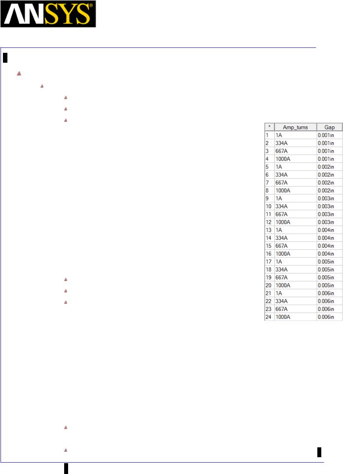
Maxwell v15

9.11

Basic Exercises – ECE: Linear Motion

Setup Parametric Analysis

To Setup Parametric Sweep

Select the menu item Maxwell 3D > Optimetrics Analysis > Add Parametric

In Setup Sweep Analysis window, on Sweep Definition tab, select Add In Add/Edit Sweep window,

1.Variable: Gap

2.Select Linear Step

3.Start: 0.001 in

4.Stop: 0.006 in

5.Step: 0.001 in

6.Select Add >>

7.Change Variable to Amp_Turns

8.Select Linear Count

9.Start: 1 A

10.Stop: 1000 A

11.Count: 4

12.Select Add >>

13.Select OK

Select Table tab to view the entire parametric table

Select Calculations tab, select Setup Calculations

In Add/Edit Calculation window,

1.Parameter: Force1

2.Category: Output Variables

3.Quantity: Fm

4.Click on Add Calculation

5.Repeat same steps for Fx, Fy and Fz

6.Change Parameter to Matrix1

7.Category: Output Variables

8.Quantity: Lcc

9.Click on Add Calculation

10.Press Done

On Options tab

1. Copy geometrically equivalent meshes:  Checked Press OK to close window

ANSYS Maxwell 3D Field Simulator v15 User’s Guide	9.11-9

Maxwell v15

9.11

Basic Exercises – ECE: Linear Motion

Solve Parametric Sweep

To Solve Parametric Analysis

Select the ParametricSetup1 tab under Optimetrics from project manager window

Right click and select Analyze

Solution Data for Parametric Sweep

To View Solution Data

Select the menu item Maxwell 3D > Optimetrics Analysis > Optimetrics Results

Create Plot of Force vs. Current for each gap

To Create Plot

Select the menu item Maxwell 3D > Results > Create Magnetostatic Report > Rectangular Plot

In Report window,

1.Parameter: Force1

2.Primary Sweep: Amp_Turns

3.Category: Output Variables

4.Quantity: Fm

5.Families: Available variations

6.Select New Report

ANSYS Maxwell 3D Field Simulator v15 User’s Guide					9.11-10

Maxwell v15

9.11

Basic Exercises – ECE: Linear Motion

ECE from the Parametric Analysis

In order to ultimately perform a system simulation in Simplorer an equivalent magnetic model must exported from Maxwell 3D. This model contains input pins for current and gap and outputs for force and flux linkage. The following steps show how to create this equivalent model. (Note: if you do not intend to do a system simulation in Simplorer, then these steps are not necessary.)

Extract Equivalent Circuit

To Extract Equivalent Circuit

Launch Simplorer and in Simplorer, select the menu item Simplorer Circuit > SubCircuit > Maxwell Component > Add Equivalent Circuit

In Maxwell Equivalent Circuit Model window,

1.Source Project File: Browse to the location of saved Maxwell Project file and select it

2.Design Type: Select 3D

3.Select the Button Extract Equivalent Circuit

Maxwell will be launched and source file will open. In Maxwell window,

1.

2.

Ensure Model Type is set to Linear Motion

Under Parametric Setup, select the parametric setup for which circuit needs to extracted

3.Select the component Z as only Z component of force will be transferred

4.Select Current Variable as Ampere-Turns as we have specified ampere-turns value for current (as we specified stranded Conductor)

5.Press Next

ANSYS Maxwell 3D Field Simulator v15 User’s Guide			9.11-11

Maxwell v15

9.11

Basic Exercises – ECE: Linear Motion

In the next window

1.As the parameters Fm, Fx and Fy will not be used in simplorer circuit, change the I/O column for these parameters to Unused

2.Make sure that the data types are correct: Gap corresponds to Position and Amp_Turns corresponds to Current.

3.Optionally if data needs to be exported in tabular format, select Export Table button

4.Press Next

Next window defines the scaling factor and the Terminals of the conservative nodes in Simplorer. The conservative nodes will have their Across and Through quantities solved by Simplorer, ensuring the physical meaning of the simulation. The Flux (and therefore the EMF) is the electrical Across quantity in this case. The current is the Through quantity. In the Mechanical domain, gap is the Across quantity whereas Force1 is the Through quantity.

In Maxwell, we specified the conductor as stranded but we have not specified number of Turns. Set Turns column for Terminal as 220 and select Finish

ANSYS Maxwell 3D Field Simulator v15 User’s Guide			9.11-12

Maxwell v15

9.11

Basic Exercises – ECE: Linear Motion

Return to Simplorer window, and select OK in the Maxwell Equivalent

Circuit Model window

Place the resulting component on the Project Page

Simplorer Circuit

Build Simplorer Circuit

Although beyond the scope of this example, build a circuit for a coupled electrical and mechanical simulation as shown below.

This coupled simulation takes into account flux linkage and back emf as well as mechanical mass and spring forces so that the closing time of the actuator can be determined.

ANSYS Maxwell 3D Field Simulator v15 User’s Guide

9.11-13

Maxwell v15

9.12

Basic Exercises – Maxwell Link with ANSYS Mechanical

Link between ANSYS Maxwell 3D and ANSYS Mechanical

This exercise describes how to set up a Maxwell 3D Eddy Current project and then link the losses to ANSYS Mechanical for a thermal calculation

3D Geometry: Iron Disk above a Spiral Coil

A sinusoidal 500 Hz current will be passed through a spiral coil which will induce eddy currents in an iron disk causing it to heat up.

Create Design

To Create Design

Select the menu item Project > Insert Maxwell 3D Design, or click on the

icon

Set Solution Type

To set the Solution Type:

Select the menu item Maxwell 3D > Solution Type

Solution Type Window:

1.Choose Magnetic > Eddy Current

2.Click the OK button

Set Model Units

To Set Units

Select the menu item Modeler > Units

In Set Modeler Units window,

1.Select units: cm (centimeters)

2.Press the OK buttom

ANSYS Maxwell 3D Field Simulator v15 User’s Guide			9.12-1

Maxwell v15

9.12

Basic Exercises – Maxwell Link with ANSYS Mechanical

Create Coil

Draw Spiral

Select the menu item Draw > User Defined Primitive > SysLib >

SegmentedHelix > PolygonHelix

In User Defined Primitive Operation window,

1.PolygonRadius: 1.5 cm

2.StartHelixRadius: 15 cm

3.RadiusChange: 3.1 cm

4.Pitch: 0 cm

5.Turns: 8

6.Leave other parameters as default and press OK

Change the name of the object to Coil and color to Yellow

Change the material of the object to Copper

Draw Box

Select the menu item Draw > Box

1. Using the coordinate entry fields, enter the box position

X: 14, Y: 0, Z: -2, Press the Enter key

2. Using the coordinate entry fields, enter the opposite corner

dX: 2, dY: 2, dZ: -2, Press the Enter key Draw another Box

Select the menu item Draw > Box

1. Using the coordinate entry fields, enter the box position

X: 40.5, Y: 0, Z: -2, Press the Enter key

2. Using the coordinate entry fields, enter the opposite corner dX: -2, dY: -2, dZ: -2, Press the Enter key

ANSYS Maxwell 3D Field Simulator v15	User’s Guide	9.12-2

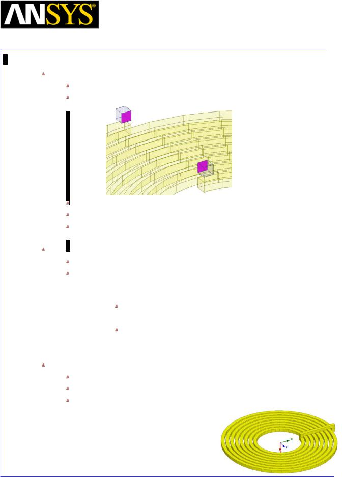
Maxwell v15

9.12

Basic Exercises – Maxwell Link with ANSYS Mechanical

Connect Surfaces

Select the menu item Edit > Select > Faces

Select the faces of the box as shown in below image

Select the menu item Modeler > Surface > Create Object from Face

Select the resulting sheet objects from the history tree

Select the menu item Modeler > Surface > Connect

Duplicate Boxes

Select Box1 and Box2 from the history tree

Select the menu item Edit > Duplicate > Along Line

1.Using the coordinate entry fields, enter the first point of duplicate vector

X: 0, Y: 0, Z: 0, Press the Enter key

2. Using the coordinate entry fields, enter the second point dX: 0, dY: 0, dZ: 1, Press the Enter key

3.Total Number: 2

4.Press OK

Unite Objects

Select the menu item Edit > Select > Objects

Select the menu item Edit > Select All

Select the menu item Modeler > Boolean > Unite

ANSYS Maxwell 3D Field Simulator v15 User’s Guide			9.12-3

			Maxwell v15		9.12
		Basic Exercises – Maxwell Link with ANSYS Mechanical
		Create Disk
		Create Regular Polyhedron
		Select the menu item Draw > Regular Polyhedron
1.			Using the coordinate entry fields, enter the center of the base
			X: 0, Y: 0, Z:1.5, Press the Enter key
2.			Using the coordinate entry fields, enter the radius
			dX: 41, dY: 0, dZ: 0, Press the Enter key
3.			Using the coordinate entry fields, enter the height
			dX: 0, dY: 0, dZ:1, Press the Enter key
4.			Number of Segments: 36

Change the name of the Object to Disk and color to Orange

Change the material of the object to cast_iron

Specify Excitations

Create Coil Terminal

Select the object Coil from the history tree

Select the menu item Modeler > Surface > Section

In Section window,

1.Section Plane: YZ

2.Press the OK button

Change the name of the resulting object to Coil_Terminal

Select the sheet Coil_Terminal from the history tree

Select the menu item Modeler > Boolean > Separate Bodies

Delete all the resulting sheets apart from Coil_Terminal

Assign Excitation

Select the object Coil_Terminal from the history tree

Select the menu item Maxwell 3D > Excitations > Assign > Current

In Current Excitation window,

1.Name: I_Coil

2.Value: 125 A

3.Type: Solid

4.Press OK

ANSYS Maxwell 3D Field Simulator v15 User’s Guide					9.12-4

Maxwell v15

9.12

Basic Exercises – Maxwell Link with ANSYS Mechanical

Resolve Skin Depth

Compute Skin Depth

Skin depth is a measure of how current density concentrates at the surface of a conductor carrying Alternating Current.

It is a function of the Permeability, Conductivity and frequency Skin Depth in meters is defined as follows:

	Where:	δ =	2
				ωσµοµr
	ω is the angular frequency, which is equal to 2πf. (f is the source
	frequency which in this case is 500Hz).
	σ is the conductor’s conductivity; for Cast Iron its 1.5e6 S/m
	µr is the conductor’s relative permeability; for Cast Iron its 60
	µ is the permeability of free space, which is equal to 4π×10-7						A/m.
		ο
	For our model the skin depth is approximately 0.24 cm.

After three skin depths, the induced current will become almost negligible. Create Surface layers to Assist with the Skin Depth Meshing

Select the menu item Edit > Select > Faces

Select the face on the disk that is closest to the coil

Select the menu item Modeler > Surface > Create Object from Face

Select the resulting sheet objects from the history tree Select the menu item Edit > Arrange > Move

1.Using the coordinate entry fields, enter the reference point of move vector

X: 0, Y: 0, Z: 0, Press the Enter key

2. Using the coordinate entry fields, enter the target point

dX: 0, dY: 0, dZ: 0.125, Press the Enter key Select the moved sheet Disk_ObjectFromFace1

Select the menu item Edit > Duplicate > Along Line

1. Using the coordinate entry fields, enter the first point

X: 0, Y: 0, Z: 0, Press the Enter key

2. Using the coordinate entry fields, enter the second point dX: 0, dY: 0, dZ:0.125, Press the Enter key

3.Total Number: 2

4.Press OK

ANSYS Maxwell 3D Field Simulator v15 User’s Guide			9.12-5

			Maxwell v15		9.12
		Basic Exercises – Maxwell Link with ANSYS Mechanical
		Define Region
		Create Simulation Region
		Select the menu item Draw > Regular Polyhedron
1.			Using the coordinate entry fields, enter the center of the base
			X: 0, Y: 0, Z:-50, Press the Enter key
2.			Using the coordinate entry fields, enter the radius
			dX: 150, dY: 0, dZ: 0, Press the Enter key
3.			Using the coordinate entry fields, enter the height
			dX: 0, dY: 0, dZ:100, Press the Enter key
4.			Number of Segments: 36

Change the name of the object to Region and Change Display Wireframe:  Checked

Set Eddy Effect

To Set Eddy Calculation for Disc

Select the menu item Maxwell 3D > Excitations > Set Eddy Effects

In Set Eddy Effects window,

1. Coil

Eddy Effects:  Unchecked

2. Disk

Eddy Effects:  Checked

Displacement Current:  Unchecked

3. Press OK

ANSYS Maxwell 3D Field Simulator v15 User’s Guide					9.12-6

Maxwell v15

9.12

Basic Exercises – Maxwell Link with ANSYS Mechanical

Analysis Setup

To create an analysis setup:

Select the menu item Maxwell 3D > Analysis Setup > Add Solution Setup

Solution Setup Window:

1. General Tab

Percentage Error: 2 2. Convergence Tab

Refinement Per Pass: 15 % 3. Solver Tab

Adaptive Frequency: 500 Hz 4. Click the OK button

Analyze

To start the solution process:

1. Select the menu item Maxwell 3D > Analyze All

Plot Mesh

To Plot Mesh on Disk

Select the object Disk from the history tree

Select the menu item Maxwell 3D > Fields > Plot Mesh

In Create Mesh Plot window, 1. Press Done

Top View	Bottom View: Notice the effect of the
	automatic adaptive meshing

ANSYS Maxwell 3D Field Simulator v15 User’s Guide	9.12-7

Maxwell v15

9.12

Basic Exercises – Maxwell Link with ANSYS Mechanical

Calculate Total Ohmic Loss

To Calculate Ohmic Losses in Disk

Select the menu item Maxwell 3D > Fields > Calculator

In Fields Calculator window,

1.Select Input > Quantity > OhmicLoss

2.Select Input > Geometry

Select Volume

Select Disk from the list

Press OK

3.Select Scalar > Integrate

4.Select Output > Eval

The evaluated value of losses in the Disk should be around 270.38 W

Plot Current Density Vectors

To Plot Current Density Vectors

Select the object Disk from the history tree

Select the menu item Maxwell 3D > Fields > Fields > J > Vector_J

In Create Field Plot window,

1.Plot on surface only:  Checked

2.Press Done

ANSYS Maxwell 3D Field Simulator v15 User’s Guide			9.12-8

Maxwell v15

9.12

Basic Exercises – Maxwell Link with ANSYS Mechanical

Plot Ohmic Loss Distribution

To Plot Ohmic Losses on Disk

Select the object Disk from the history tree

Select the menu item Maxwell 3D > Fields > Fields > Other > Ohmic_Loss

In Create Field Plot window,

1.Plot on surface only:  Checked

2.Press Done

This is the end of the Maxwell 3D Eddy Current Design

Save and Exit

Save the file

Select the menu item File > Save As

Save the file with the name “Ex_9_12_BasicEddy_ANSYS_thermal” Select the menu item File > Exit

ANSYS Maxwell 3D Field Simulator v15 User’s Guide			9.12-9

Maxwell v15

9.12

Basic Exercises – Maxwell Link with ANSYS Mechanical

ANSYS Mechanical

In this section of tutorial, we will map the losses calculated by Maxwell to ANSYS Mechanical Steady State Thermal Solver. Solution in ANSYS Mechanical will give final temperature distribution of the objects.Mapping data from Maxwell to ANSYS Mechanical will be done through Workbench interface

Launch ANSYS Workbench

To Launch ANSYS Workbench

Select the Microsoft Start button and Select Programs > ANSYS 14.0 >

Workbench

ImportMaxwell File

To Import Maxwell Project

In Workbench Project window, select the menu item File > Import

Set the file type to Maxwell Project File

Browse to the file Ex_9_12_BasicEddy_ANSYS_thermal.mxwl and Open it A Maxwell 3D Design is created as shown below

Create ANSYS Mechanical Design

To Create Steady State Thermal Design

Select a Steady State Thermal Analysis System from Analysis Systems list

Drag and drop it on the Solution tab of Maxwell 3D Design

Similarly drag and drop the Geometry tab of Maxwell on the Geometry tab of Steady State Thermal system. This will create a link between Maxwell Solution and Setup of ANSYS Mechanical

Right click on Solution tab of Maxwell 3D Design and Select Update to update the solution cell

Right click on the Geometry tab of Steady State Thermal system and select Refresh

ANSYS Maxwell 3D Field Simulator v15 User’s Guide					9.12-10

Maxwell v15

9.12

Basic Exercises – Maxwell Link with ANSYS Mechanical

Define Material Database

To Define Material Database

Right click on the tab Engineering Data and select Edit

In Engineering Data window,

1. Select the icon Engineering Data Sources

2.Select the tab Thermal Materials from Data Sources

3.Locate Cast Iron material from the list and select Add

Launch ANSYS Mechanical

To Launch ANSYS Mechanical

Right click on Model tab of Steady State Thermal analysis system and select Edit

A tab corresponding to Maxwell data is automatically added in the tree to enable data mapping

ANSYS Maxwell 3D Field Simulator v15 User’s Guide					9.12-11

Maxwell v15

9.12

Basic Exercises – Maxwell Link with ANSYS Mechanical

Setup Geometry

Suppress Unwanted Objects

Expand the Project tree for Geometry under Model

Select all bodies apart from Disk, right click on the Bodies and select Suppress

This will keep only Disk for analysis and rest will be ignored

Specify Material

Select the Disk from the tree and goto Details View window

In Details View window, 1. Material

Assignment: set to Cast Iron

ANSYS Maxwell 3D Field Simulator v15 User’s Guide							9.12-12

Maxwell v15

9.12

Basic Exercises – Maxwell Link with ANSYS Mechanical

Generate Mesh

Mesh specifications are important from the data mapping perspective. The mesh should be sufficiently refined in order to have good accuracy in mapped heat losses from Maxwell to ANSYS Mechanical

To Set Mesh Parameters

Right click on Mesh tab from specification tree and select Insert > Method In Details View window,

1.Geometry: select the body Disk

2.Method: Sweep

3.Sweep Num Divs: 5

This will ensure four elements across the thickness of the disk and give the refinement close to the mesh we have in Maxwell

To Generate Mesh

Right click on Mesh tab and select Generate Mesh

ANSYS Maxwell 3D Field Simulator v15 User’s Guide			9.12-13

Maxwell v15

9.12

Basic Exercises – Maxwell Link with ANSYS Mechanical

Map Data from Maxwell

To Map Heat Loss Data from Maxwell

Right click on the Imported Load (Maxwell3DSolution) and select Insert > Heat Generation

In Details View window,

1. Geometry: Select the body Disk

Right click on the tab Imported Heat Generation and select Import Load

Heat losses calculated in Maxwell be mapped to the mesh in ANSYS Mechanical

A Summery of mapped heat losses is shown below Imported Heat Generation tab. Scaling factor shown in this summery should be close to 1 to ensure correct data mapping. If not, mesh needs to be refined in important regions

Specify Convective Boundary

To Specify Convective Boundary

Right click on Steady State Thermal tab from the specification tree and select Insert > Convection

In Details View window, 1. Geometry:

Change Selection Filter to Faces

Right click in Graphic window and select Select All

Press Apply in details view window 2. Film Coefficient: 10 W/m2°C

ANSYS Maxwell 3D Field Simulator v15 User’s Guide					9.12-14

Maxwell v15

9.12

Basic Exercises – Maxwell Link with ANSYS Mechanical

Create Temperature Plot

To Create Temperature Plot for Disk

Right click on Solution tab from specification tree and select Insert > Thermal > Temperature

Solve

To Run the Solution

Right click on Solution tab from specification tree and select Solve

Temperature Plot

To View Temperature Plot

Select the Temperature plot from specification tree under Solution Temperature distribution on Disk will be displayed in graphic window

ANSYS Maxwell 3D Field Simulator v15 User’s Guide					9.12-15

Maxwell v15

9.13

Basic Exercises – Transient – Large Motion - Rotational

Large Motion – its Quick Implementation Using the Maxwell 3D Transient Solver

Maxwell Transient is able to consider interactions between transient electromagnetic fields and mechanical motion of objects.

Maxwell Transient (with motion) includes dB /dt arising from mechanically moving magnetic fields in space, i.e. moving objects. Thus, effects coming from so-called motion induced currents can be considered.

In Maxwell rotational motion can occur around one single motion axis.

This paper represents a quick start to using rotational motion. It will exercise rotational motion in Maxwell 3D using a rotational actuator (experimental motor) example.

Subsequent papers will demonstrate rotational motion in more depth, noncylindrical rotational motion using a relays example, as well as translational motion which a solenoid application will serve as an example for.

The goal of these papers is solely to show and practice working with large motion in Maxwell. It is neither the goal to simulate real-world applications, nor to match accurately measured results, nor will these papers show in detail how to setup and work with other Maxwell functionality. Please refer to the corresponding topics.

Quickstart – Rotational Motion Using a Rotational Actuator Example

Maxwell Transient with large motion is a set of advanced topics. Users should have thorough knowledge on Maxwell fundamentals as well as Maxwell Transient (without motion) prior to approaching large motion. If necessary, please consult the proper training papers, help files, manuals, and application notes.

We will exercise the following in this document:

Create a new or read in an existing rotational actuator model – to serve as an experimental testbench for large motion

Prepare and adapt this existing actuator model to our needs

Apply large motion to the rotational actuator

Create the band object

Setup rotational motion Mesh

ANSYS	Maxwell 3D Field Simulator v15 User’s Guide					9.13-1

Maxwell v15

9.13

Basic Exercises – Transient – Large Motion - Rotational

Perform basic large motion tests

“Large Rotational Standstill” test

“Large Rotational Constant Speed” test

“Large Rotational Transient Motion” test

Compute magnetic rigidity and mechanical natural frequency

Estimate timestep for transient solver

Make a field animation with large motion

Open Input File

To Open the file

Select the menu item File > Open

Browse to the file Ex_9_13_Large_Motion_Rotational.mxwl and open it File should look as shown below

ANSYS Maxwell 3D Field Simulator v15 User’s Guide			9.13-2

Maxwell v15

9.13

Basic Exercises – Transient – Large Motion - Rotational

Setup and Verify the Electromagnetic Part

Prior to employing large motion, the electromagnetic part of the model should work correctly. Users are well advised not to setup a complex model completely at once and then try to simulate. Rather, they should work in steps. Especially in cases where the model includes eddy current effects, external circuits, and large motion, extra steps should be taken to verify the correctness of the setup for each individual property. After that, all properties can be considered together.

We use stranded windings with constant current (to generate a fixed stator flux vector around which Rotor1 will oscillate later). Also, eddy effects will be excluded.

Perform a test simulation on the electromagnetic part alone. If desired, play with various excitations, switch eddy effects in Stator1 and Rotor1 on and off, vary material properties, etc. For each test check the electromagnetic fields for correctness.

Refer to the corresponding topics on materials, boundaries, excitations, meshing, transient simulations without motion, and post processing.

If the electromagnetic part without motion effects yielded correct results, make sure to re-apply the same model setup as elaborated at the previous page

Rotational Large Motion – The Maxwell Approach

Maxwell separates moving from non-moving objects.

All moving objects must be enclosed by one so-called band object.

For rotational motion, the band object must be cylindrical with segmented outer surface, i.e. a regular polyhedron.

Maxwell considers all moving objects (inside the band) to form one single moving object group.

Constant Speed mode:

If the model is setup to operate in constant speed mode (see below), Maxwell will not compute mechanical transients.

However, changing magnetic fields owing to speed ωm, i. e. dB/dt effects are included in the field solution.

Mechanical Transient mode:

In case inertia was specified, Maxwell will compute the motion equation in each time step.

J	m	· d2ϕ (t) / dt2	+	k	(t) · dϕ (t) / dt =	T (t)	+ T (t)
		m		D	m	ψ	m

See Appendix A for a variable explanation.

ANSYS Maxwell 3D Field Simulator v15 User’s Guide	9.13-3

Maxwell v15

9.13

Basic Exercises – Transient – Large Motion - Rotational

Setup Model

First, let‘s examine the moving parts to comply with Maxwell‘s conventions:

All moving objects can be separated from the stationary objects and can be combined to one single rotating group. All moving objects be considered to perform the same cylindrical motion.

However, the band object has a hole that we have to fill first.

Because there is only one moving object, there is no immediate need to enclose it. But filling the hole can also be achieved by fully enclosing Rotor1 by an extra object. We will first do this.

Create Enclosure for Rotor

Outer radius of Rotor is around 51.05 mm and height is 25.4 mm

Select the menu item Draw > Cylinder

1. Using the coordinate entry fields, enter the center of the base

X: 0, Y: 0, Z: 0, Press the Enter key

2. Using the coordinate entry fields, enter the radius

dX: 51.05, dY: 0, dZ: 0, Press the Enter key 3. Using the coordinate entry fields, enter the height

dX: 0 dY: 0, dZ: 25.4, Press the Enter key

Change the name of the resulting object to Region_Inner and material to Vacuum

Note: Instead of using coordinate entry field, users can directly pick vertices of Rotor to specify radius and height directly.

ANSYS Maxwell 3D Field Simulator v15 User’s Guide			9.13-4

Maxwell v15

9.13

Basic Exercises – Transient – Large Motion - Rotational

Create Band Object

We want a regular polyhedron that fully encloses Region_Inner.

Outer surface segmentation should be between 1° and 5°, i. e. we will have between 360 and 72 outer surface segments.

The band object should preferably cut through the middle of the airgap, leaving about the same space to Rotor1 and Stator1. However, this is not a must.

Inner radius of the Stator is around 53.75 mm while outer radius of Rotor is around 51.05 mm

Thus middle position comes out to be 52.4 mm. So we will use 52.5 mm as radius of Band object

Select the menu item Draw > Regular Polyhedron

1. Using the coordinate entry fields, enter the center of the base

X: 0, Y: 0, Z: -12.5, Press the Enter key

2. Using the coordinate entry fields, enter the radius

dX: 52.5, dY: 0, dZ: 0, Press the Enter key 3. Using the coordinate entry fields, enter the height

dX: 0, dY: 0, dZ:50, Press the Enter key 4. Number of Segments: 72

Change the name of the object to Band and material to Vacuum

ANSYS Maxwell 3D Field Simulator v15 User’s Guide					9.13-5

Maxwell v15

9.13

Basic Exercises – Transient – Large Motion - Rotational

Setup1: Large Rotational Standstill Assign Motion

To Specify Motion

Select the object Band from the history tree

Select the menu item Maxwell 3D > Model > Motion Setup > Assign Band

In Motion Setup window, Type tab

1.Motion Type: Rotation

2.Rotation Axis: Global:Z

3.Positive:  Checked

Data tab

1. Initial Position: 0 deg

Thus, motion will start at t = 0 with the rotor position being as drawn. A ϕm0 ≠ 0 would start with Rotor1 rotated by ϕm0 from the drawn position.

2. Rotate Limit:  Unchecked Mechanical tab

1.Consider Mechanical Transient:  Unchecked

2.Angular Velocity: 0 rpm

Press OK

Now, we have setup “Large Rotation Standstill“ Positive magnetic torque is generated around the positive z-axis (global coordinate system)

A mesh Operation is automatically created after motion setup which will ensure refinement of mesh in the gap region between Band and Stator/Rotor

Analysis Setup

To Create Analysis Setup

Select the menu item Maxwell 3D > Analysis Setup > Add Solution Setup

In Solve Setup window,

1.Stop Time: 20 ms

2.Time Step: 5 ms

3.Press OK

ANSYS Maxwell 3D Field Simulator v15 User’s Guide					9.13-6

Maxwell v15

9.13

Basic Exercises – Transient – Large Motion - Rotational

Mesh Operations

Meshing is a very critical issue with respect to simulation speed and accuracy. For here, we will apply a rather coarse mesh only, by which the solver will just yield satisfactory results.

To Assign Mesh Operations on Band

For torque computation, the most critical areas are the airgap and its immediate proximity. Thus, the band mesh is crucial for accurate results.

Our Band1 is 50 mm high, one segment is about 4.5 mm wide.

We will apply a length based mesh on the surface and inside of Band1. Tetrahedral edge length will be set to 20 mm. We will then see a mesh length of about 10 mm on the outer surface. This will do for these tests.

Select the object Band from the history tree

Select the menu item Maxwell 3D > Mesh Operations > Assign > Inside Selection > Length Based

In Element Length Based Refinement window,

1.Name: Band_Length

2.Restrict Length of Elements:  Checked

3.Maximum Length of Elements: 20 mm

4.Restrict the Number of Elements:  Unchecked

5.Press OK

To Assign Mesh Operations on other Objects

Press Ctrl and select the objects CoilA and CoilB

Select the menu item Maxwell 3D > Mesh Operations > Assign > Inside Selection > Length Based

In Element Length Based Refinement window,

1.Name: Coils_Length

2.Restrict Length of Elements:  Checked

3.Restrict the Number of Elements:  Unchecked

4.Maximum Number of Elements: 1000

5.Press OK

Note: Simultaneously selecting CoilA and CoilB will try to assign 1000 tetrahedrals to both objects, i. e. about 500 to each

ANSYS Maxwell 3D Field Simulator v15 User’s Guide					9.13-7

Maxwell v15

9.13

Basic Exercises – Transient – Large Motion - Rotational

In Similar way specify Mesh operations of other objects as specified below

Region_Inner

1.Name: Region_Inner_Length

2.Maximum Number of Elements: 2000

Rotor

1.Name: Rotor_Length

2.Maximum Number of Elements: 2000

Stator

1.Name: Stator_Length

2.Maximum Number of Elements: 2000

Region

1.Name: Region_Length

2.Maximum Number of Elements: 2500

To Create Mesh

Select the menu item Maxwell 3D > Analysis Setup > Apply Mesh Operations

Select all the objects except Region and select the menu item Maxwell 3D > Fields > Plot Mesh

ANSYS Maxwell 3D Field Simulator v15 User’s Guide			9.13-8

Maxwell v15

9.13

Basic Exercises – Transient – Large Motion - Rotational

Run Solution

To Run the Solution

Select the menu item Maxwell 3D > Analyze All

Results

Create Plot for Torque

Select the menu item Maxwell 3D > Results > Create Transient Report > Rectangular Plot

In Reports window,

1.Solution: Setup1: Transient

2.Parameter: Moving1

3.X: Default

4.Category: Torque

5.Quantity: Torque

6.Press New Report

Report should show a constant torque value of 0.4Nm

ANSYS Maxwell 3D Field Simulator v15 User’s Guide					9.13-9

Maxwell v15

9.13

Basic Exercises – Transient – Large Motion - Rotational

Setup2 : Large Rotational Constant Speed

We will now operate the rotational actuator at a very slow constant speed.

Remember, there is only one magnetic excitation present in the model – namely constant coil current with stranded windings. Alternatively, Rotor1 could have been assigned permanent magnet properties. Eddy effects have been switched off for all objects.

We can now use Transient with Large Motion to monitor cogging torque effects.

Copy Design

To Craete a Copy of Design

Select the tab Large_Motion_Standstill from the Project manager window, right click and select Copy

Right click on the Project Name in Project Manager window and select Paste

Change the name of the design to Large_Motion_ConstantSpeed

ModifyRotation Specifications

To Modify Rotation

Expand the tree for Model from Project Manager window

Double click on MotionSetup1 to open Motion Setup window

In Motion Setup window,

Data tab

1. Change Initial Position to -61 deg Mechanical tab

1. Change Angular Velocity to 1 deg_per_sec Press OK

Rotor as drawn has a -29° offset. This is taken to be the zero position for the transient solver. By giving an extra -61°, positive rotation of 1 °/s starts at -90°.

ANSYS Maxwell 3D Field Simulator v15 User’s Guide	9.13-10

Maxwell v15

9.13

Basic Exercises – Transient – Large Motion - Rotational

Modify Solution Setup

To Modify Solver Setup

Expand the tree for Analysis from Project manager window

Double click on Setup1 to open Solve Setup window

In Solve Setup window,

1.Change Stop Time to 180 s

2.Chnage Time Step to 5 s

3.Press OK

By rotating at a speed of 1 °/s 180 s long, Rotor will move 180°, i. e. from - 90° to +90°, at 5°/step.

Run Solution

To Run the Solution

Select the menu item Maxwell 3D > Analyze All

Results

To View Plot

Expand the tree for Results from Project Manager window

Double click on Torque plot that was created previously

ANSYS Maxwell 3D Field Simulator v15 User’s Guide					9.13-11

Maxwell v15

9.13

Basic Exercises – Transient – Large Motion - Rotational

Setup3 : Large Rotational Transient Motion

We will now operate the actuator as a one-body oscillator.

Inertia will be specified as well as some damping.

We can expect Rotor to oscillate around the stator flux axis (y-axis) at some natural frequency f0, which can be approximated as:

f	0	=	1			cψ
			2π			J

J in kgm2 is the total moment of inertia acting on Rotor.

cψ in Nm/rad is the magnetic rigidity. As an analogy it can be understood as a mechanical spring spanned between Rotor and Stator, whose force coming from the magnetic field.

We can roughly calculate rigidity c from the cogging torque function (stable limb):

cψ = ∆Tψ ≈ 400 mNm = 2.3 Nm/rad ∆ϕm rad(10°)

Assuming inertia J = 0.0024 kgm2, an approximated f0 = 5 Hz results.

This is sufficient for estimating the necessary timestep as far as mechanical oscillations are regarded.

Copy Design

To Craete a Copy of Design

Select the tab Large_Motion_ConstantSpeed from the Project manager window, right click and select Copy

Right click on the Project Name in Project Manager window and select Paste

Change the name of the design to Large_Motion_MechTransient

ANSYS Maxwell 3D Field Simulator v15 User’s Guide					9.13-12

Maxwell v15

9.13

Basic Exercises – Transient – Large Motion - Rotational

Modify Rotation Specifications

To Modify Rotation

Expand the tree for Model from Project Manager window

Double click on MotionSetup1 to open Motion Setup window

In Motion Setup window,

Data tab

1. Change Initial Position to 0 deg Mechanical tab

1.Consider Mechanical Transient:  Checked

2.Initial Angular Velocity: 0 deg_per_sec

3.Moment of Inertia: 0.0024 Kgm^2

4.Damping: 0.015 N-m-sec/rad

5.Load Torque: 0 NewtonMeter

Press OK

This causes 15 mNm resistive torque at 1 rad/s speed

We thus expect oscillation between -29° and +29° (w. r. t. stator flux axis) at f0 < 5 Hz with damped amplitudes

Modify Solution Setup

To Modify Solver Setup

Expand the tree for Analysis from Project manager window

Double click on Setup1 to open Solve Setup window

In Solve Setup window,

1.Change Stop Time to 0.5 s

2.Chnage Time Step to 0.01 s

3.Press OK

From f0, we can expect a >200 ms cycle. At 10 ms timestep we will sample one cycle >20 times.

ANSYS Maxwell 3D Field Simulator v15 User’s Guide			9.13-13

Maxwell v15

9.13

Basic Exercises – Transient – Large Motion - Rotational

Run Solution

To Run the Solution

Select the menu item Maxwell 3D > Analyze All

Results

To View Torque Plot

Expand the tree for Results from Project Manager window

Double click on Torque plot that was created previously

To Create Plots for Speed and Position

Select the menu item Maxwell 3D > Results > Create Transient Report > Rectangular Plot

In Reports window,

1.Solution: Setup1: Transient

2.Parameter: Moving1

3.X: Default

4.Category: Speed

5.Quantity: Speed

6.Press New Report

ANSYS Maxwell 3D Field Simulator v15 User’s Guide					9.13-14

Maxwell v15

9.13

Basic Exercises – Transient – Large Motion - Rotational

Plot for Speed should look as below

In Reports window,

1.Change Category to Position

2.Quantity: Position

3.Press New Report

ANSYS Maxwell 3D Field Simulator v15 User’s Guide					9.13-15

Maxwell v15

9.13

Basic Exercises – Transient – Large Motion - Rotational

Appendix A: Variable Explanation:

ϕm(t)

ϕm0

dϕm(t) / dt, ωm(t)

ωm0

d2ϕm(t) / dt2 Jm

kD(t)

Tψ

Tm

t

Mechanical angular position in rad (angles can also be given in degrees).

Initial ϕm in rad. Note that the drawn rotor position is considered as ϕm0 = 0.

Mechanical angular speed in rad/s. Initial ωm in rad/s.

Mechanical angular acceleration in rad/s2.

Moment of inertia in kg·m2. This is the total inertia acting on the moving object group. If extra inertia needs to be included (i. e. inertia not geometrically modeled), just add this to Jm.

Damping koefficient in Nm·s/rad. For kD = 1 Nm·s/rad, resistive torque of 1 Nm would be generated if the moving parts turn at 1 rad/s. kD can be a function of t, ωm, or ϕm.

Magnetically generated torque in Nm.

Mechanical extra torque in Nm, this can be a constant or a function of t, ωm, or ϕm. Note, that a positive Tm value will accelerate rather than brake.

The current simulation time in s.

ANSYS Maxwell 3D Field Simulator v15 User’s Guide					9.13-16

Maxwell v15

9.14

Basic Exercises – Electric Transient Solver

Introduction on the Electric Transient Solver

This note introduces the Electro Transient solver based on a simple example. This solver is meant to solve the transient electric field with current flowing in “real” dielectrics before they reach electrostatic equilibrium.

Practical applications for an electric transient solver range from low frequency biomedical applications to fine aspects of electric conduction in poor conductors, both insulators and semi-conductors. Charge relaxation is often of interest. Other application areas are distribution of electric fields in LED arrays, study of (transient) electric fields in insulators, effects related to non-linear conductivity materials used to control electric field stress in high voltage applications.

Maxwell’s Capacitor

In this example, we want to determine the transient electric field in the two layers of “real” dielectric material between two plates connected to a voltage source. Material properties in the two layers of dielectric are uniform within each layer but different between the two layers. We do not need to draw the plates; we just need to draw the two media regions.

Create Design

To Create Design

Select the menu item Project > Insert Maxwell 3D Design, or click on the

icon

Set Solution Type

To set the Solution Type:

Select the menu item Maxwell 3D > Solution Type

Solution Type Window:

1. Choose Electric > Electric Transient

2. Click the OK button

ANSYS Maxwell 3D Field Simulator v15 User’s Guide	9.14-1

			Maxwell v15			9.14
			Basic Exercises – Electric Transient Solver
		Define Settings
		To set Maxwell Settings
		Select the menu item Tools > Options > Maxwell 3D Options
		In Maxwell 3D Options window,
1.			General Options tab
					Default insulator/conductor: 1e-9 siemens/m
2.			Click the OK button

Create Geometry

Create Box_Bottom

Select the menu item Draw > Box

1. Using the coordinate entry fields, enter the box position

X: -1, Y: -2, Z: -0.6, Press the Enter key

2. Using the coordinate entry fields, enter the opposite corner

dX: 2, dY: 4, dZ: 0.6, Press the Enter key

Change the name of the Object to Box_Bottom

Create Box_Top

Select the object Box_Bottom from the history tree Select the menu item Edit > Duplicate > Along Line

1.Using the coordinate entry fields, enter the first point of duplicate vector

X: 0, Y: 0, Z: 0, Press the Enter key

2. Using the coordinate entry fields, enter the opposite corner dX: 0, dY: 0, dZ: 0.6, Press the Enter key

3.Total Number: 2

4.Press OK

Change the name of the Object to Box_Top

ANSYS Maxwell 3D Field Simulator v15	User’s Guide	9.14-2

Maxwell v15

9.14

Basic Exercises – Electric Transient Solver

Create Materials

To Create Material for Box_Bottom

Select the object Box_Bottom, right click and select Assign Material In Select Definition window,

1.Select Add Material

2.In View/Edit Material window,

Material Name: Mat_Bottom

Relative Permittivity: 5

Bulk Conductivity: 1e-7 siemens/m

Select OK

To Create Material for Box_Top

Select the object Box_Top, right click and select Assign Material

In Select Definition wondow,

1.Select Add Material

2.In View/Edit Material window,

Material Name: Mat_Top

Relative Permittivity: 4

Bulk Conductivity: 2e-8 siemens/m

Select OK

Assign Excitations

We apply the voltage to the plates. We did not draw the plates, because we can apply a voltage to the top and bottom part of the regions.

Assign Excitation for Box_Top

Select the menu item Edit > Select > Faces

Select the top face of the object Box_Top

Select the menu item Maxwell 3D > Excitations > Assign > Voltage

In Voltage Excitation window,

1.Set Value to if(Time<0, 0, if(Time<2.5e-3,1,0))

2.Press OK

Select the bottom face of the object Box_Bottom

Select the menu item Maxwell 3D > Excitations > Assign > Sink

In Sink Excitation window, 1. Press OK

ANSYS Maxwell 3D Field Simulator v15	User’s Guide	9.14-3

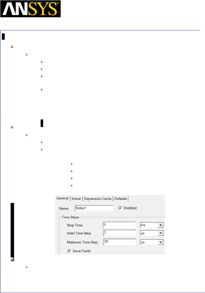
Maxwell v15

9.14

Basic Exercises – Electric Transient Solver

Assign Mesh Operations

To Assign Mesh operations

Select the menu item Edit > Select > Objects

Press Ctrl and select the objects Box_Bottom and Box_Top

Select the menu item Maxwell 3D > Mesh Operations > Assign > Inside Selection > Length Based

In Element Length Based Refinement window,

1.Restrict length of Elements:  Checked

2.Maximum Length of Elements: 0.55 mm

3.Press OK

Analysis Setup

To create an analysis setup:

Select the menu item Maxwell 3D > Analysis Setup > Add Solution Setup

Solution Setup Window:

1. General Tab

Stop Time: 5 ms

Initial Time Step: 1us

Maximum Time Step: 10 us Save Fields:  Checked

2. Click the OK button

Analyze

To start the solution process:

1. Select the menu item Maxwell 3D > Analyze All

ANSYS Maxwell 3D Field Simulator v15 User’s Guide					9.14-4

Maxwell v15

9.14

Basic Exercises – Electric Transient Solver

Create Objects for Plots

Create a Point

Select the menu item Draw > Point

1. Using the coordinate entry fields, enter the point position

X: 0, Y: 0, Z: 0.3, Press the Enter key

Create another Point

Select the menu item Draw > Point

1. Using the coordinate entry fields, enter the point position X: 0, Y: 0, Z: -0.3, Press the Enter key

Create Parameters for Plot

To Create Parameters

Select the menu item Maxwell 3D > Fields > Calculator

1.Select Input > Quantity > E

2.Select Vector > Scal? > ScalarZ

3.Select Input > geometry

Select Point

Select Point1 from the list

Press OK

4.Select Output > Value

5.Press Add

6.Specify name of the parameter as E_a and press OK

7.Select Input > Quantity > E

8.Select Vector > Scal? > ScalarZ

9.Select Input > geometry

Select Point

Select Point2 from the list

Press OK

10.Select Output > Value

11.Press Add

12.Specify name of the parameter as E_b and press OK

13.Press Done

ANSYS Maxwell 3D Field Simulator v15 User’s Guide					9.14-5

Maxwell v15

9.14

Basic Exercises – Electric Transient Solver

Create Plot

To Create Plot

Select the menu item Maxwell 3D > Results > Create Field Report > Rectangular Plot

In Report window,

X: Default

Category: Calculator Expressions

Quantity: E_a

Select New Report

Change Quantity to E_b Select Add Trace

Plot E_Vector on a Plane

To Plot E_Vector

Expand the tree for Planes from history tree and select the plane Global:XZ

Select the menu item Maxwell 3D > Fields > Fields > E > E_vector

In Create Field Plot window,

1.Instrinsic Variables >Time:1e-6 sec

2.Press Done

ANSYS Maxwell 3D Field Simulator v15 User’s Guide					9.14-6

			Maxwell v15		9.14
			Basic Exercises – Electric Transient Solver
		Modify Plot Attributes
		Double click on the Legend to modify plot attributes
		In the window,
1.			Marker/Arrow tab
			Arrow Options
			1. Size : move to right to increase arrow length
2.			Plot tab
			Vector Plot

1.Spacing: move to left to reduce space between arrows

3.Press Apply and Close

Animate Plot

To Animate Plot

Expand the tree for Field Overlays from Project Manager window

Select the plot E_Vector1 from the list, right click and select Animate In Setup Animation window, set start time and Stop Time and press OK

ANSYS Maxwell 3D Field Simulator v15 User’s Guide			9.14-7

Maxwell v15

9.14

Basic Exercises – Electric Transient Solver

System level Simulation

Due to uniform thickness of the dielectric layer, the surface of separation between the two dielectrics can be assumed to be equipotential. Thus it becomes possible to replace the two dielectric layers with equivalent series/parallel RC circuits shown in the next page.

Since the material and geometry information of the two dielectric layers are known, the resistances and capacitances can be calculated with the equations:

,

Comparison of the voltages across the dielectric layers simulated in a circuit/system level simulator and calculated in Maxwell

ANSYS Maxwell 3D Field Simulator v15 User’s Guide					9.14-8

Maxwell v15

9.15

Basic Exercises – PM Assignment

Hallbach Array

This exercise will discuss how to set up a Hallbach array consisting of 5 magnets. This procedure is applicable for Magnetostatic and Transient Solvers.

Problem definition

We are interested to solve the magnetic field around a Hallbach array consisting of 5 magnets. The magnetization direction of each magnet is shown below. The dimensions of each magnet are 5, 10, and 20 mm, respectively. The permanent magnet material is N27 (Br = 1.03T; Hc = 796 kA/m).

Create Design

To Create Design

Select the menu item Project > Insert Maxwell 3D Design, or click on the

icon

Set Solution Type

To set the Solution Type:

Select the menu item Maxwell 3D > Solution Type

Solution Type Window:

1.Choose Magnetic > Magnetostatic

2.Click the OK button

ANSYS Maxwell						9.15-1
	3D Field Simulator v15 User’s Guide

Maxwell v15

9.15

Basic Exercises – PM Assignment

Create Geometry

Draw Box

Select the menu item Draw > Box

1. Using the coordinate entry fields, enter the box position

X: 0, Y: 0, Z: 0, Press the Enter key

2. Using the coordinate entry fields, enter the opposite corner

dX: 10, dY: 20, dZ: 5, Press the Enter key

Change the name of the resulting object to Magnet1

Duplicate Box

Select the object Magnet1 from the history tree Select the menu item Edit > Duplicate > Along Line

1.Using the coordinate entry fields, enter the first point of duplicate vector

X: 0, Y: 0, Z: 0, Press the Enter key

2. Using the coordinate entry fields, enter the second point

dX: 10, dY: 0, dZ: 0, Press the Enter key 3. Total Number: 5

Change the name of the resulting object to Magnet2 through Magnet5 in positive Y direction

ANSYS Maxwell 3D Field Simulator v15 User’s Guide			9.15-2

Maxwell v15

9.15

Basic Exercises – PM Assignment

Check Orientation of Objects

Each object in Maxwell is associated with certain coordinate system. This is called Orientation and it is specified under attributes for each object. The Orientation of a newly created (or imported) object is Global.

To Check Orientation of Magnet1

Select the object Magnet1 from the history tree, right click and select Properties

A Properties window will pop up where Orientation of the object is listed

Here Magnet1 is orientated with respect to Global coordinate system

By left clicking on Global, we can change the orientation of the object to any other existing coordinate system

Another way to Check Orientation

Select the menu item Tools > Options > Modeler Options

In Modeler Options window, 1. Display tab

Show orientation of selected objects:  Checked 2. Press OK

This will enable display of coordinate system in small for each select object. The displayed coordinate system will the one to which object is oriented

ANSYS Maxwell 3D Field Simulator v15 User’s Guide							9.15-3

Maxwell v15

9.15

Basic Exercises – PM Assignment

Define Permanent Magnet

The magnet material is N27, which does not exist in the library. We have to create a new material with the properties of N27. For permanent magnets with the linear characteristic in the second quadrant (such as N27), the demagnetization curve is approximated with a line. This line is uniquely defined by specifying Remanence Br (1.03) and Coercive Field Hc (796 kA/m).

To Define Magnet Material

Press Ctrl and select the objects Magnet1 through to Magnet5

Right click and select Assign Material In Select Definition window,

1.Type NdFe35 in the Search by Name field

2.Select Clone Material button

In View/Edit Material window,

1.

2.

3.

Material Name: N27

Select the tab Calculate Properties for Permanent Magnet In Properties for Permanent Magnet window,

Mu:  Unchecked

Hc:  Checked

Specify value of -796000

Br/Mp:  Checked

Br: 1.03 Press OK

4.Note that the Relative Permeability (slope of the line) is automatically determined from the equation of the line defined by Br and Hc.

5.Press OK to create material N27

ANSYS Maxwell 3D Field Simulator v15 User’s Guide							9.15-4

Maxwell v15

9.15

Basic Exercises – PM Assignment

The direction of magnetization is specified by a unit vector relative to the Coordinate System (CS) associated with the given object, that is relative to the Orientation of the object. If the Orientation of the object is Global, the unit vector will be specified relative to the Global CS. Maxwell also allows to specify the type of the Coordinate System (upper right corner ). Thus Cartesian, Cylindrical and Spherical CS type can be defined. This means that if the Orientation of the object is Global and CS type Cartesian, the unit vector will be specified as X, Y, and Z relative to the Cartesian Global CS.

Hence, the right direction of magnetization is specified by the appropriate combination of object’s Orientation, CS type and Unit Vector.

For this particular magnet definition, the unit vector is [1,0,0]. This means that if the magnet remains oriented in the Global CS, the magnet will be magnetized in the Global X direction.

In order to change this direction, we either change the unit vector or define a new coordinate system and associate the magnet with it. The X-axis of the new CS will have point in the direction of magnetization as the original (default) unit vector [1,0,0] in this case remains unchanged.

The most advantageous is creation of FACE coordinate systems, which is discussed in the following.

ANSYS Maxwell 3D Field Simulator v15 User’s Guide					9.15-5

Maxwell v15

9.15

Basic Exercises – PM Assignment

Create Orientation CS

In this step, face coordinate systems are created in order to specify orientation of each magnet with respect to them.

While creating FaceCS, it is ensured that X direction of the resulting CS is pointing in the direction of magnetization of corresponding object.

To Create FaceCS for Magnet1

Select the menu item Edit > Select > Faces

Select the face of Magnet1 as shown in below image

Select the menu item Modeler > Coordinate System > Create > FaceCS

For the origin of the new face CS, snap to the face center (cursor becomes circle) and click

For the X-axis (note that this should be oriented downwards in order to be aligned with the magnetization direction of magnet1) snap to the center of bottom edge (cursor becomes triangle) and click.

X-axis of the newly created face CS is now aligned with the direction of magnetization of Magnet1

ANSYS Maxwell 3D Field Simulator v15 User’s Guide							9.15-6

Maxwell v15

9.15

Basic Exercises – PM Assignment

Expand the history tree for Coordinate Systems and select FaceCS1

Goto the properties window and change the name of the coordinate system as Magnet1_N

Note also that small red W next to CS name signifies current working CS. Clicking on Global, Global CS again becomes current CS.

The above procedure for face CS creation has to be repeated for each magnet. At the end we have 5 face CS:

ANSYS Maxwell 3D Field Simulator v15 User’s Guide					9.15-7

Maxwell v15

9.15

Basic Exercises – PM Assignment

Set Orientation CS for Objects

Select the object Magnet1 from the history tree

Right click and select Properties

Change the Orientation from Global to Magnet1_N

In similar way, set the orientation of each object with respect to their

FaceCS

ANSYS Maxwell 3D Field Simulator v15 User’s Guide					9.15-8

Maxwell v15

9.15

Basic Exercises – PM Assignment

Define Region

Create Simulation Region

Select the menu item Draw > Region

In Region window,

1.Pad all directions similarly:  Checked

2.Padding Type: Absolute Offset

3.Value: 50mm

4.Press OK

Analysis Setup

To create an analysis setup:

Select the menu item Maxwell 3D > Analysis Setup > Add Solution Setup

Solution Setup Window:

1. General Tab

Maximum Number of Passes: 20 2. Click the OK button

Analyze

To start the solution process:

1. Select the menu item Maxwell 3D > Analyze All

ANSYS	Maxwell 3D Field Simulator v15 User’s Guide			9.15-9

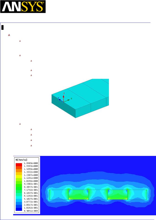
Maxwell v15

9.15

Basic Exercises – PM Assignment

Results

We will plot the magnetic flux density on the magnets’ middle plane. In order to access this plane, we have to create a new coordinate system such that one plane associated with this CS will be coincident with magnets’ middle plane.

To Create CS

Select the menu item Modeler > Coordinate System > Create > Relative CS > Offset

Snap cursor to any magnet’s middle point

XZ plane of this new CS is coincident with magnets’ middle plane

ToCreate Filed Plot

Exapnd the history tree for Planes

Select the plane RelativeCS1:XZ

Select the menu item Maxwell 3D > Fileds >Fields > B > Mag_B

In Create Field Plot window, 1. Press Done

ANSYS Maxwell 3D Field Simulator v15 User’s Guide					9.15-10

Maxwell v15

9.16

Basic Exercises – Electric Transient (High Voltage Line)

Overview

This exercise explains how an electric transient case can be solved using Maxwell V15.

The exercise uses the example of a high voltage electric line. The electric field between the line and the ground is simulated with Electric Transient Solver

As the Electric Transient solver does not provide adaptive meshing, we will first solve the case using Electrostatic solver and import its adaptively refined mesh for use in Transient solution

Launch Maxwell

To Launch Maxwell

To access Maxwell, click the Microsoft Start button, select Programs, and select Ansoft and then Maxwell 15.

Open Input File

To open a file

In Maxwell window, select the menu item File Open.

Browse to the file “Ex_9_16_BasicElectricTransient_HighVoltageLine.mxwl” and select Open

The file contains the geometry of the power line termination created in Maxwell as shown in below image. The geometry contains a copper conductor surrounded by insulating objects. The materials for all the object is already set in the file. Conductor and ground terminals are specified with copper material

ANSYS Maxwell 3D Field Simulator v15 User’s Guide					9.16-1

Maxwell v15

9.16

Basic Exercises – Electric Transient (High Voltage Line)

Set Solution Type

The case will be solved with the Electrostatic solver to get an adaptively refined mesh. The refined mesh will be used for the transient solution

To set the solution type

Select the menu item Maxwell 3D > Solution Type

Solution Type Window:

1.Choose Electrostatic

2.Click the OK button

Create Excitations

Specify excitation for the Conductor

Select the object Conductor from the tree

Go to the menu item Maxwell 3D > Excitations > Assign > Voltage

In the Voltage Excitation Window

1.Name: High_Voltage

2.Value: 175 kV

3.Click the OK button

ANSYS Maxwell 3D Field Simulator v15 User’s Guide							9.16-2

Maxwell v15

9.16

Basic Exercises – Electric Transient (High Voltage Line)

Specify excitation for Ground

Select the object Ground from the history tree

Go to the menu item Maxwell 3D > Excitations > Assign > Voltage

In the Voltage Excitation Window

1.Name: Ground

2.Value: 0 V

3.Click the OK button

Specify excitation for Shield

Select the object Ground from the history tree

Go to the menu item Maxwell 3D > Excitations > Assign > Voltage

In the Voltage Excitation Window

1.Name: Shield_Ground

2.Value: 0 V

3.Click the OK button

Analysis Setup

To Create an Analysis Setup

Go to the menu item Maxwell 3D > Analysis Setup > Add Solution Setup

In the Solve Setup window

1.General tab

•Percentage Error: 1

2.Convergence tab

•Refinement Per Pass: 15 %

3.Press OK to close

ANSYS Maxwell 3D Field Simulator v15 User’s Guide					9.16-3

Maxwell v15

9.16

Basic Exercises – Electric Transient (High Voltage Line)

Save Project

To save the project:

In an Ansoft Maxwell window, select the menu item File > Save As.

From the Save As window, type the appropriate file name Click the Save button

Model Validation

To validate the model:

Select the menu item Maxwell 3D > Validation Check

Click the Close button

Note: To view any errors or warning messages, use the Message

Manager.

Analyze

To start the solution process:

Select the menu item Maxwell 3D > Analyze All

ANSYS Maxwell 3D Field Simulator v15 User’s Guide			9.16-4

Maxwell v15

9.16

Basic Exercises – Electric Transient (High Voltage Line)

Plot Mesh

To Hide Region

Press Ctrl and select the objects InnerRegion and Region

Select the menu item View > Hide Selection > Active View

To Plot Mesh

Select the menu item Edit > Select All Visible

Select the menu item Maxwell 3D > Fields > Plot Mesh

In Create Mesh Plot window,

Press Done

Copy Design

To Create a Copy of the Design

Select the design “Design_Nominal” from the Project Manager tree, right click and select “Copy”

Select the tab “Ex_9_16_BasicElectricTransient_HighVoltageLine” in Project Manager tree, right click and select “Paste”

Rename the newly created design as “Design_Transient”

Set Transient Solution

To Set Transient Solution Type

Double click on “Design_Transient” from the Project manager window to activate it

Select the menu item Maxwell 3D > Solution Type

In Solution Type window

1.Change Solution Type to Electric >Transient

2.Press OK

ANSYS Maxwell 3D Field Simulator v15 User’s Guide					9.16-5

			Maxwell v15	9.16
		Basic Exercises – Electric Transient (High Voltage Line)
		Transient Analysis Setup
		To Create a Transient Analysis Setup
		Go to Maxwell 3D > Analysis Setup > Add Solution Setup
		In Solve Setup Window
1.			General Tab
			Stop Time: 6 ns
			Initial Time Step: 0.05 ns
			Maximum Time Step: 0.5 ns
2.			Solver Tab
			Import mesh:  Checked
			In Setup Link Window

1. Source Project: Use This Project  Checked

2. Source Design: Design_Nominal

3. Press OK

ANSYS Maxwell 3D Field Simulator v15 User’s Guide						9.16-6

Maxwell v15

9.16

Basic Exercises – Electric Transient (High Voltage Line)

Model Validation

To validate the model

Select the menu item Maxwell 3D > Validation Check

Click the Close button

Analyze

To start the solution process:

Select the menu item Maxwell 3D > Analyze All

Rectangular Plot

Create a point to plot magnitude of E on it

Select the menu item Draw > Point

1. Using Coordinate Entry Field, Enter the point position X: 0, Y: 0, Z: -150, Press Enter

ANSYS Maxwell 3D Field Simulator v15 User’s Guide									9.16-7

Maxwell v15

9.16

Basic Exercises – Electric Transient (High Voltage Line)

To Plot Mag_E Vs Time

Select the menu item Maxwell 3D > Results > Create Field Reports >

Rectangular Plots

In Report window,

1.Geometry: Point1

2.X : Default

3.Category: Calculator Expressions

4.Quantity: Mag_E

5.Select New Report

Plot will be displayed on the screen

From the plot, it is clear that the magnitude of E has reached steady value by 6ns and field has developed completely. Thus the solution need not to be run further

ANSYS Maxwell 3D Field Simulator v15 User’s Guide					9.16-8

Maxwell v15

9.16

Basic Exercises – Electric Transient (High Voltage Line)

Mag_E Field Plot

Plot Mag_E at Time= 0s

Select Global: XZ plane from the history tree

Go to Maxwell 3D > Fields > Fields > E > Mag_E

In the Create Filed Plot window

1.Time: 0 s

2.Select Done

Similarly create a plot at Time = 6e-9 s

To Change the Plot Attributes

Double click on the legend to modify plot

In the window

1.Scale tab

2.Num. Divisions: 50

3.Log:  Checked

4.Press Apply and Close

ANSYS Maxwell	3D Field Simulator v15 User’s Guide			9.16-9

Maxwell v15

9.16

Basic Exercises – Electric Transient (High Voltage Line)

A Field Plot will be displayed on screen as shown below

Plot at Time = 0s

Plot at Time = 6e-9s

ANSYS Maxwell 3D Field Simulator v15 User’s Guide			9.16-10

Maxwell v15

9.16

Basic Exercises – Electric Transient (High Voltage Line)

Voltage Field Plot

Plot Voltage at Time= 0s

Select Global: XZ plane from the history tree

Go to Maxwell 3D > Fields > Fields > Voltage

In the Create Filed Plot window

1.Time: 0 s

2.Select Done

Similarly create a plot of Voltage at Time = 6e-9s

Time = 0s

Time = 6e-9s

ANSYS Maxwell 3D Field Simulator v15 User’s Guide	9.16-11

Maxwell v15

10.0

Chapter 10.0 – Optimetrics

Chapter 10.0 – Optimetrics

10.1 – Gapped Inductor

ANSYS Maxwell 3D Field Simulator v15 User’s Guide							10.0

Maxwell v15

10.1

Example (Optimetrics) – Gapped Inductor

Gapped Inductor

This example describes how to create and optimize a gapped inductor for a particular value of inductance using the 3D Magnetostatic solver and Optimetrics in the ANSYS Maxwell 3D Design Environment.

Two optimizations will be completed:

1.Obtain the desired inductance by varying current

2.Obtain the desired inductance by core gap

ANSYS Maxwell 3D Field Simulator v15 User’s Guide							10.1-1

Maxwell v15

10.1

Example (Optimetrics) – Gapped Inductor

ANSYS Maxwell Design Environment

The following features of the ANSYS Maxwell Design Environment are used to

create the models covered in this topic

3D Solid Modeling

Primitives: Box, Recatangle

Boolean Operations: Subtract, Unite, Separate Bodies

Boundaries/Excitations

Current: Stranded

Analysis

Magnetostatic

Optimetrics

Results

Inductance

Flux Density

ANSYS Maxwell 3D Field Simulator v15 User’s Guide					10.1-2

Maxwell v15

10.1

Example (Optimetrics) – Gapped Inductor

Launching Maxwell

To access Maxwell:

1.Click the Microsoft Start button, select Programs, and select Ansoft > Maxwell 15.0 and select Maxwell 15.0

Setting Tool Options

To set the tool options:

Note: In order to follow the steps outlined in this example, verify that the following tool options are set :

1. Select the menu item Tools > Options > Maxwell 3D Options

Maxwell Options Window:

1. Click the General Options tab

Use Wizards for data input when creating new boundaries:  Checked

Duplicate boundaries/mesh operations with geometry:

Checked

2.Click the OK button

2.Select the menu item Tools > Options > Modeler Options.

Modeler Options Window:

1. Click the Operation tab

Automatically cover closed polylines:  Checked 2. Click the Display tab

Default transparency = 0.8 3. Click the Drawing tab

Edit property of new primitives:  Checked 4. Click the OK button

ANSYS Maxwell 3D Field Simulator v15 User’s Guide					10.1-3

Maxwell v15

10.1

Example (Optimetrics) – Gapped Inductor

Opening a New Project

To open a new project:

After launching Maxwell, a project will be automatically created. You can also create a new project using below options.

1.In an Maxwell window, click the  On the Standard toolbar, or select the menu item File > New.

Select the menu item Project > Insert Maxwell 3D Design, or click on the icon

Set Solution Type

To set the Solution Type:

Select the menu item Maxwell 3D > Solution Type

Solution Type Window:

1.Choose Magnetostatic

2.Click the OK button

Set Model Units

To Set the units:

Select the menu item Modeler > Units

Set Model Units:

1.Select Units: mm

2.Click the OK button

ANSYS	Maxwell 3D Field Simulator v15 User’s Guide			10.1-4

Maxwell v15

10.1

Example (Optimetrics) – Gapped Inductor

Create EECore

Create a Box

Select the menu item Draw > Box

1. Using the coordinate entry fields, enter the position of box

X: -10, Y: -20, Z: -10, Press the Enter key

2. Using the coordinate entry fields, enter the opposite corner

dX: 20, dY: 40, dZ: 20, Press the Enter key

Change Attributes

Select the resulting object from the history tree and goto Properties window

1.Change the name of the object to Core

2.Change the color of the object to Gray

3.Change the material of the object to “mu_metal”

Select the menu item View > Fit All > Active View

Create Core window

Select the menu item Draw > Box

1. Using the coordinate entry fields, enter the position of box

X: -10, Y: -15, Z: -5, Press the Enter key

2. Using the coordinate entry fields, enter the opposite corner

dX: 20, dY: 10, dZ: 10, Press the Enter key Change Attributes

Select the resulting object from the history tree and goto Properties window 1. Change the name of the object to Window

Duplicate Window

Select the object Window from the history tree Select the menu item, Edit > Duplicate > Along Line

1.Using the coordinate entry fields, enter the first point of duplicate vector

X: 0, Y: 0, Z: 0, Press the Enter key

2. Using the coordinate entry fields, enter the second point dX: 0, dY: 20, dZ: 0, Press the Enter key

3.Total Number: 2

4.Press OK

ANSYS Maxwell 3D Field Simulator v15 User’s Guide			10.1-5

Maxwell v15

10.1

Example (Optimetrics) – Gapped Inductor

Subtract Windows from Core

Select the menu item Edit > Select All

Select the menu item Modeler > Boolean > Subtract

In Subtract window,

1.Blank Parts: Core

2.Tool Parts: Window, Window_1

3.Press OK

Create Coil

Create a Box

Select the menu item Draw > Box

1. Using the coordinate entry fields, enter the position of box

X: -18, Y: -13, Z: -4, Press the Enter key

2. Using the coordinate entry fields, enter the opposite corner

dX: 36, dY: 26, dZ: 8, Press the Enter key

Change Attributes

Select the resulting object from the history tree and goto Properties window

1.Change the name of the object to Coil

2.Change the color of the object to Red

3.Change the material of the object to “copper”

Create Hole

Select the menu item Draw > Box

1. Using the coordinate entry fields, enter the position of box

X: -11, Y: -6, Z: -4, Press the Enter key

2. Using the coordinate entry fields, enter the opposite corner

dX: 22, dY: 12, dZ: 10, Press the Enter key Change Attributes

Select the resulting object from the history tree and goto Properties window 1. Change the name of the object to Hole

ANSYS Maxwell 3D Field Simulator v15 User’s Guide			10.1-6

Maxwell v15

10.1

Example (Optimetrics) – Gapped Inductor

Subtract Hole from Coil

Press Ctrl and select the objects Coil and Hole from history tree

Select the menu item Modeler > Boolean > Subtract

In Subtract window,

1.Blank Parts: Coil

2.Tool Parts: Hole

3.Press OK

Create Coil Terminal

Create Section of coil

Select the object Coil from the history tree

Select the menu item Modeler > Surface > Section

In Section window,

1.Section Plane: YZ

2.Click the OK button

Change Attributes

Select the object Coil_Section1 from the tree and goto Properties window 1. Change the name of the object to Coil_Terminal

Separate Sheets

Select the sheet Coil_Terminal

Select the menu item Modeler > Boolean > Separate Bodies

Delete Extra Sheets

Select the sheet Coil_Terminal_Seperate1 from the tree Select the menu item Edit >Delete

Create Core Gap

To Create Core gap

Select the menu item Draw > Box

1. Using the coordinate entry fields, enter the position of box

X: -15, Y: -25, Z: 0, Press the Enter key

2. Using the coordinate entry fields, enter the opposite corner dX: 30, dY: 50, dZ: 0.1, Press the Enter key

ANSYS Maxwell	3D Field Simulator v15 User’s Guide					10.1-7

Maxwell v15

10.1

Example (Optimetrics) – Gapped Inductor

Change Attributes

Select the resulting object from the history tree and goto Properties window 1. Change the name of the object to Gap

Parameterize Gap

Expand the history tree for the object Gap

Double click on the command CreateBox from the history tree In Properties window,

1.For ZSize type gap, press Tab to accept the value

2.In Add Variable window,

Unit Type: Length

Unit: mm

Value: 0.1

Press OK

3. Press OK to close Properties window Subtract Gap from Core

Press Ctrl and select the objects Coil and Hole from history tree

Select the menu item Modeler > Boolean > Subtract

In Subtract window,

1.Blank Parts: Core

2.Tool Parts: Gap

3.Press OK

Separate Core

It is necessary to unlump both core halves for inductance calculation

Select the object Core from the history tree

Select the menu item Modeler > Boolean > Separate Bodies

Core_Separate1 will be created.

Rename the object as Core2

ANSYS Maxwell 3D Field Simulator v15 User’s Guide					10.1-8

Maxwell v15

10.1

Example (Optimetrics) – Gapped Inductor

Define Region

Create Simulation Region

Select the menu item Draw > Region

In Region window,

1.Pad all directions similarly:  Checked

2.Padding Type: Percentage Offset

3.Value: 50

4.Press OK

Assign Excitations

To Assign Excitations

Select the object Coil_Terminal from the history tree

Select the menu item Maxwell 3D > Excitations > Assign > Current

In Current Excitation window,

1.Name: Current1

2.Value: ampturns

3.Type: Stranded

4.Press OK

In Add Variable window,

1.Unit Type: Current

2.Unit: A

3.Value: 100

4.Press OK

Calculate Inductance

To Assign Inductance Calculation

Select the menu item Maxwell 3D > Parameters > Assign > Matrix

In matrix window,

Current1

Include:  Checked

Press OK

ANSYS Maxwell	3D Field Simulator v15 User’s Guide					10.1-9

Maxwell v15

10.1

Example (Optimetrics) – Gapped Inductor

Analysis Setup

To create an analysis setup:

Select the menu item Maxwell 3D > Analysis Setup > Add Solution Setup

Solution Setup Window: 1. General tab

Maximum Number of Passes: 5 2. Press OK

Note: Convergence will not be very good with specified settings. The settings are used just to demonstrate the optimetrics capabilities in faster way.

Save Project

To save the project:

1.In an Ansoft Maxwell window, select the menu item File > Save As.

2.From the Save As window, type the Filename: Ex_10_1_Core_Inductance

3.Click the Save button

ModelValidation

To validate the model:

Select the menu item Maxwell 3D > Validation Check

Click the Close button

Note: To view any errors or warning messages, use the Message Manager.

Analyze

To start the solution process:

1. Select the menu item Maxwell 3D > Analyze All

ANSYS Maxwell 3D Field Simulator v15 User’s Guide			10.1-10

Maxwell v15

10.1

Example (Optimetrics) – Gapped Inductor

Solution Data

To view the Solution Data:

Select the menu item Maxwell 3D > Results > Solution Data

To view the Profile:

1. Click the Profile Tab. To view the Convergence:

1. Click the Convergence Tab

Note: The default view is for convergence is Table. Select the Plot radio button to view a graphical representations of the convergence data.

To View Mesh information

1. Click the Mesh Statistics tab

To view the Inductance values: 1. Click the MatrixTab

ANSYS Maxwell 3D Field Simulator v15 User’s Guide					10.1-11

Maxwell v15

10.1

Example (Optimetrics) – Gapped Inductor

Plot Flux Density in the core

To Hide Region

Select the object Region from the history tree

Select the menu item View > Hide Selection > Active View

To Plot Flux Density

Expand the history tree for Planes and select Global: YZ

Select the menu item Maxwell 3D > Fields > Fields > B > Mag_B

In Create Field Plot window,

1.Quantity: Mag_B

2.In Volume: Press Ctrl and select Core and Core2

3.Press Done

Note: This field plot is for the nominal design case with gap = 0.1mm and ampturns = 100A.

ANSYS Maxwell 3D Field Simulator v15 User’s Guide							10.1-12

Maxwell v15

10.1

Example (Optimetrics) – Gapped Inductor

Optimetrics Setup and Solution

It is possible to optimize current, material properties such as permeability, or any geometric dimension such as gap in order to obtain the specified inductance. For this optimization, the current will be varied to obtain the desired inductance of 0.8uH. Later, the gap will be varied to obtain the desired inductance

Specify Parametric Variables

Select the menu item Maxwell 3D > Design properties

In Properties window,

1.

2.

Optimization:  Checked gap:

Include:  Checked

Min : 0.05 mm Max : 1 mm

3. ampturns:

Include:  Checked

Min : 1 A

Max : 500 A 4. Press OK

ANSYS Maxwell 3D Field Simulator v15 User’s Guide			10.1-13

Maxwell v15

10.1

Example (Optimetrics) – Gapped Inductor

Setup an Optimization Analysis

Select the menu item Maxwell 3D > Optimetrics Analysis > Add

Optimization

In Setup Optimization window,

1.Optimizer: Sequential Nonlinear Programming

2.Max. No. of Iterations: 20

3.Select Setup Calculations

4.In Add/Edit calculations window, select Output Variables

5.In Output variables window,

Name: target

Expression: 8e-7 H

Select Add

Without closing window, set name to cost1

Parameter: Matrix1

Expression: abs(target - L(Current1,Current1))/target/1H

Note: In the same Output Variable window, enter cost function. This unitless cost function is the absolute value of the percent difference between the desired inductance (target) and the calculated inductance (L(Current1,Current1)). Cost1 will approach zero as the calculated inductance approaches the desired inductance.Use Insert Into Expression buttons to help build this equation.

Press Add and Done

6. In Add/Edit Calculations window,

Parameter : Matrix1

Category: Output Variables

Quantity: cost1

Select Add Calculation Press Done

ANSYS Maxwell 3D Field Simulator v15 User’s Guide					10.1-14

Maxwell v15

10.1

Example (Optimetrics) – Gapped Inductor

7.Parameter cost1 will be added to Setup Optimization window.

8.Set Condition for cost1 to Minimize

9.Change the tab to Variables

10.For the variable ampturns

Override:  Checked

Include:  Checked

Max Focus: 200 11. For the variable gap

Override:  Checked Include:  Unchecked

12. Change the tab to Options

Save Fields And Mesh:  Checked

Copy geometrically equivalent meshes:  Checked

13. Press OK to close the window.

ANSYS Maxwell 3D Field Simulator v15 User’s Guide					10.1-15

Maxwell v15

10.1

Example (Optimetrics) – Gapped Inductor

Solve Optimization Analysis

To Solve Optimization Analysis

Select the menu item Maxwell 3D > Analyze All

View Optimetrics Results

To View Results

Select the menu item Maxwell 3D > Optimetrics Analysis > Optimetrics Results

In Post Analysis Display window, 1. Log Scale:  Checked

Plot Display should look as below

Change View to Table to see actual values

Press Close

ANSYS Maxwell 3D Field Simulator v15 User’s Guide	10.1-16

Maxwell v15

10.1

Example (Optimetrics) – Gapped Inductor

Create Plot of Cost vs Ampturns

To create a report:

Select the menu item Maxwell 3D > Results > Create Magnetostatic Report > Rectangular Plot

In Report window,

1.Parameter: Matrix1

2.Primary Sweep: ampturns

3.Category: Output Variables

4.Quantity: cost1

5.Select New Report

6.Press the Close button

The minimum cost occurs at 178 A

ANSYS Maxwell 3D Field Simulator v15 User’s Guide					10.1-17

Maxwell v15

10.1

Example (Optimetrics) – Gapped Inductor

Second Optimetrics Setup and Solution

For the second optimization, the core gap will be varied to obtain the desired inductance of 0.8uH with ampturns = 100A.

Setup Optimization Analysis

To Setup an Optimization Analysis

Select the menu item Maxwell 3D > Optimetrics Analysis > Add

Optimization

In Setup Optimization window,

1.Optimizer: Sequential Nonlinear Programming

2.Max. No. of Iterations: 20

3.Select Setup Calculations

4.In Add/Edit Calculations window,

Parameter : Matrix1

Category: Output Variables

Quantity: cost1

Select Add Calculation

Press Done

5.Set Condition for cost1 to Minimize

6.Change the tab to Variables

7.For the variable gap

Include:  Checked 8. For the variable ampturns Starting value: 100 A

Include:  Unchecked 9. Change the tab to Options

Save Fields And Mesh:  Checked 10. Press OK

ANSYS Maxwell 3D Field Simulator v15 User’s Guide			10.1-18

Maxwell v15

10.1

Example (Optimetrics) – Gapped Inductor

Solve Optimization Analysis

To Solve Optimization Analysis

Exand the Project Manager tree to see Optimetrics

Right click on Optimization Setup2 and select Analyze

View Optimetrics Results

To View Results

Right click on the tab Optimization Setup2 from Project Manager tree and select View Analysis Results

In Post Analysis Display window, 1. Log Scale:  Checked

Plot Display should look as below

Change View to Table to see actual values

Press Close

ANSYS Maxwell 3D Field Simulator v15 User’s Guide			10.1-19

Maxwell v15

10.1

Example (Optimetrics) – Gapped Inductor

Create Plot of Cost vs gap

To create a report:

Select the menu item Maxwell 3D > Results > Create Magnetostatic Report > Rectangular Plot

In Report window,

1.Parameter: Matrix1

2.Primary Sweep: gap

3.Category: Output Variables

4.Quantity: cost1

5.Change tab to Families

6.Under Sweeps, for variable ampturns, Select Edit

Use all values:  Unchecked

Select the value 100 A

Select Close

7.Select New Report

8.Press the Close button

ANSYS Maxwell 3D Field Simulator v15 User’s Guide			10.1-20

Maxwell v15

10.1

Example (Optimetrics) – Gapped Inductor

Minimum value of cost occurs at around 195 μm

In similar way, plot Inductance Vs Gap

From the plot it can be seen that target value of 0.8 uH for inductance is achieved at a gap of 220 μm

ANSYS Maxwell 3D Field Simulator v15 User’s Guide			10.1-21

	Maxwell v15		11.0
		Chapter 11.0 – Motors

Chapter 11.0 – Motors

11.1 – Motor Application Notes

ANSYS Maxwell 3D Field Simulator v15 User’s Guide							11.0

	Maxwell v15		11.1
		Motor Application Note

Study of a Permanent Magnet Motor with MAXWELL 3D:

Example of the 2004 Prius IPM Motor

ANSYS Maxwell 3D Field Simulator v15 User’s Guide			11.1-1

	Maxwell v15		11.1
		Motor Application Note

Study of a Motor

The Electro Mechanical software package provided by Ansoft enables extensive motor simulation. This application note details the simulaton of a motor with Maxwell3D. We will cover static and transient simulations.

This application note will use the 2004 Toyota Prius motor as basis. It is a 8- pole permanent magnet motor with embedded magnets. The single layer windings are made of 3 phases. The stator has 48 slots. This motor is public, we therefore have the full set of parameters. We will also use Oak Ridge National Laboratory testing results in this note.

Note: This application has not been done with the collaboration of Toyota

References:

Report on Toyota/Prius Motor Torque Capability, Torque Property, No-Load Back EMF, and Mechanical Losses,

J. S. Hsu, Ph.D., C. W. Ayers, C. L. Coomer, R. H. Wiles

Oak Ridge National Laboratory

Report on Toyota/Prius Motor Design and manufacturing Assessment

J. S. Hsu, C. W. Ayers, C. L. Coomer

Oak Ridge National Laboratory

Evaluation of 2004 Toyota Prius Hybrid Electric Drive System Interim Report

C. W. Ayers, J. S. Hsu, L. D. Marlino, C. W. Miller,G. W. Ott, Jr.,C. B. Oland Oak Ridge National Laboratory

ANSYS Maxwell 3D Field Simulator v15 User’s Guide							11.1-2

	Maxwell v15		11.1
		Motor Application Note

Overview of the Study:

Getting Started

Launching Maxwell

Setting Tool Options

Opening a new project

Set Model Units

Creating the 3D Model

Create the Stator

Create the Rotor

Create the Magnets

Create the Windings

Reducing the size of the 3D Model

Material properties of the motor

Permanent Magnets characterization

Steel definition

Applying Master/Slave Boundary Condition

STATIC ANALYSIS

Full Load Study

Apply Excitations

Apply Mesh Operations

Apply Torque computation

Inductance computation

Analyze Setup

Analyze

Postprocessing

ANSYS Maxwell 3D Field Simulator v15 User’s Guide			11.1-3

	Maxwell v15		11.1
		Motor Application Note

Overview of the Study (Cont’d)

DYNAMIC ANALYSIS

Create Current Terminals

Motor Excitation

Create Parameters for excitations

Create Windings

Add Band object

Mesh Operations

Assign Movement

Add an Analysis Setup

Solve the problem

Post Processing

Parametric Study

ANSYS Maxwell 3D Field Simulator v15 User’s Guide			11.1-4

	Maxwell v15		11.1
		Motor Application Note

Getting Started

Launching Maxwell

1.To access Maxwell, click the Microsoft Start button, select Programs, and select Ansoft and then Maxwell 15.0 and Maxwell15.0

Setting Tool Options

To set the tool options:

Note: In order to follow the steps outlined in this example, verify that the following tool options are set :

1.Select the menu item Tools > Options > Maxwell 3D Options

2.Maxwell Options Window:

1. Click the General Options tab

Use Wizards for data entry when creating new boundaries:  Checked

Duplicate boundaries with geometry:  Checked

2.Click the OK button

3.Select the menu item Tools > Options > Modeler Options.

4.3D Modeler Options Window:

1.Click the Operation tab

Automatically cover closed polylines:  Checked 2. Click the Drawing tab

Edit property of new primitives:  Checked 3. Click the OK button

ANSYS Maxwell 3D Field Simulator v15 User’s Guide			11.1-5

	Maxwell v15		11.1
		Motor Application Note

Opening a New Project

To open a new project:

In an Maxwell window, click the  icon on the Standard toolbar, or select the menu item File > New.

Right mouse click on the project name, then select the menu item Rename. Change the project name to Ex_11_1_PriusMotor

Select the menu item Project > Insert Maxwell Design, or click on the icon

Right mouse click on Maxwelldesign1 and select Rename. Change the name to 1_Whole_Motor

Set Model Units

To Set Model Units

Select the menu item Modeler > Units.

1.Select Units: mm (millimeters)

2.Press OK

ANSYS Maxwell 3D Field Simulator v15 User’s Guide			11.1-6

	Maxwell v15		11.1
		Motor Application Note

Creating the 3D Model

Maxwell has number of User Defined Primitives for motor parts. These primitives can describe all the main parts of motors.

Create the Stator:

A User Defined Primitive will be used to create the stator

Select the menu item Draw > User Defined Primitive > Syslib > Rmxprt > SlotCore

Use the values given in the panel below to create the stator

ANSYS Maxwell 3D Field Simulator v15 User’s Guide			11.1-7

Maxwell v15

11.1

Motor Application Note

Change Attributes

Change the name of the object to Stator

Change the color of the object to Gray

Create the Rotor

A User Defined Primitive will be used to create the rotor

Select the menu item Draw > User Defined Primitive > Syslib > Rmxprt > IPMCore

Use the values given in the below to create the rotor

ANSYS Maxwell 3D Field Simulator v15 User’s Guide							11.1-8

	Maxwell v15		11.1
		Motor Application Note

Change Attributes

Change the name of the object to Rotor

Change the color of the object to Green

Create the Magnets

The same User Defined Primitive can be used to create the magnets, but with different parameters. UDPs can be computed to generate different topologies.

Select the menu item Draw > User Defined Primitive > Syslib > Rmxprt > IPMCore

Use the values given in the panel below to create the magnets

ANSYS Maxwell 3D Field Simulator v15 User’s Guide			11.1-9

Maxwell v15

11.1

Motor Application Note

Change Attributes

Change the name of the object to Magnet

Change the color of the object to Light Red

Create Windings

A User Defined Primitive will be used to create the windings.

Select the menu item Draw > User Defined Primitive > Syslib > Rmxprt > LapCoil

Use the values given in the panel below to create the coil Change Attributes

Change the material of the object to Copper Change the color of the object to Yellow

ANSYS Maxwell 3D Field Simulator v15 User’s Guide									11.1-10

Maxwell v15

11.1

Motor Application Note

Rotate Coil

Select the object LapCoil1 from the history tree

Select the menu item Edit > Arrange > Rotate

In Rotate window,

1.Axis: Z

2.Angle: 7.5 deg

3.Press OK

Duplicate Coil

Select the object LapCoil1 from the history tree

Select the menu item Edit > Duplicate > Around Axis

In Duplicate Around Axis window,

1.Axis: Z

2.Angle : 15 deg

3.Total Number: 3

4.Press OK

Change Attributes

Change the name of the objects LapCoil1, LapCoil1_1 and LapCoil1_2 to PhaseA, PhaseC, and PhaseB respectively

Change the color of the objects PhaseB and Phase C to Blue and Red

ANSYS Maxwell	3D Field Simulator v15 User’s Guide			11.1-11

	Maxwell v15		11.1
		Motor Application Note

Duplicate Coils

Press Ctrl and select the object PhaseA, PhaseB and PhaseC from the history tree

Select the menu item Edit > Duplicate > Around Axis

In Duplicate Around Axis window,

1.Axis: Z

2.Angle : 45 deg

3.Total Number: 8

4.Press OK

Motor geometry is complete

ANSYS Maxwell 3D Field Simulator v15 User’s Guide			11.1-12

	Maxwell v15		11.1
		Motor Application Note

Copy Design

To Copy Design

Select the Maxwell design “1_Whole_Motor” from the Project Manager tree, right click and select “Copy”

Select the project name from the Project manager tree, right click and select “Paste”

Change the name of the design to “2_Partial_Motor”

Reduce Model Size

We can take advantage of the topology of the motor to reduce the size of the problem. This motor has 8 pair of poles. We can only use one height of the motor. This is valid because the stator has:

48 slots (8 is a divider of 48).

The 3-phase winding has also a periodicity of 45 degrees.

From now on, the Maxwelldesign ‘2_Partial_motor’ will be used. We have saved a copy of the whole geometry as it will be used later for other studies.

Rotate Model

Press Ctrl and select the object Stator and all Coils

Select the menu item Edit > Arrange > Rotate

In Rotate window,

1.Axis: Z

2.Angle: 7.5 deg

3.Press OK

This will shift the winding before splitting the objects.

Split Model by XZ

Select the menu item Edit > Select All

Select the menu item Modeler > Boolean > Split

In Split window,

1.Split Plane: XZ

2.Keep fragments: Positive Side

3.Split Objects: Split entire Selection

4.Press OK

ANSYS Maxwell 3D Field Simulator v15 User’s Guide					11.1-13

Maxwell v15

11.1

Motor Application Note

Rotate Model

We have achieved half model now

Select the menu item Edit > Select All

Select the menu item Edit > Arrange > Rotate

In Rotate window,

1.Axis: Z

2.Angle: -45 deg

3.Press OK

Split Model by XZ

Select the menu item Edit > Select All

Select the menu item Modeler > Boolean > Split

In Split window,

1.Split Plane: XZ

2.Keep fragments: Negative Side

3.Split Objects: Split entire Selection

4.Press OK

Rotate Model

Select the menu item Edit > Select All

Select the menu item Edit > Arrange > Rotate

In Rotate window,

1.Axis: Z

2.Angle: 45 deg

3.Press OK

Split Model by XY

Select the menu item Edit > Select All

Select the menu item Modeler > Boolean > Split

In Split window,

1.Split Plane: XY

2.Keep fragments: Positive Side

3.Split Objects: Split entire Selection

4.Press OK

ANSYS Maxwell 3D Field Simulator v15 User’s Guide					11.1-14

	Maxwell v15		11.1
		Motor Application Note

Reduced Model

The 3D model now looks like below

Change Attributes

Change the name of the objects PhaseA and PhaseA_7 to PhaseA1 and PhaseA2

Change the name of the objects PhaseB_7 to PhaseB1

Change the name of the object PhaseC and PhaseC_7 to PhaseC1 and PhaseC2

Create Region

Create Rectangle

Select the menu item Modeler > Grid Plane > XZ

Select the menu item Draw > Rectangle

1. Using the coordinate entry field, enter the box position

X: 0.0, Y: 0.0, Z: 0.0, Press the Enter key

2. Using the coordinate entry field, enter the relative size of the box dX: 200.0, dY: 0.0, dZ: 100.0, Press the Enter key

ANSYS Maxwell 3D Field Simulator v15 User’s Guide					11.1-15

Maxwell v15

11.1

Motor Application Note

Sweep Rectangle

Select the sheet Rectangle1 from the history tree

Select the menu item Draw > Sweep > Around Axis

In Sweep Around Axis window,

1.Axis: Z

2.Angle of sweep: 45

3.Number of segments: 5

4.Press OK

Change Attributes

Change the name of the object to Region

Select Display Wireframe:  Checked

ANSYS Maxwell 3D Field Simulator v15 User’s Guide					11.1-16

	Maxwell v15		11.1
		Motor Application Note

Material Properties for the Motor

Permanent Magnet Characterization

The Prius Permanent Magnets (PMs) are high-strength magnets.

In order to define PMs magnetization orientation, we need to create separate objects for each magnet.

Separate Objects

Select the object Magnets from the history tree

Select the menu item Modeler > Boolean > Separate Bodies

Change Attributes

Change the name of the object Magnets to PM1

Change the name of the object Magnets_Separate1 to PM2

Since the magnets will rotate, the orientation cannot be given through fixed coordinate systems (CS). The use of face CS is required. Face CS are CS that are attached to the face of an object. When the object moves, the Face CS also moves along with the object.

The Prius’s PMs are oriented as shown below. Therefore, we will create a face CS for each magnet.

ANSYS Maxwell 3D Field Simulator v15 User’s Guide					11.1-17

	Maxwell v15		11.1
		Motor Application Note

Hide All other Objects

Select the menu item View > Visibility > Active View Visibility

In the window,

1.Disable the visibility for all objects except Rotor, PM1 and PM2

2.Press Done

To Create Face Coordinate System

Select the menu item Edit > Select > Faces or press “f” from keyboard

Select the top face of the object PM1 as shown in below image

Select the menu item Modeler > Coordinate System > Create > Face CS

Select the vertex on the top face of PM1 to define origin

Select the vertex of the magnet as shown in below image to define X axis

A Face coordinate system will be created as shown in below image

Rename the FaceCS1 to PM1_CS

ANSYS Maxwell 3D Field Simulator v15 User’s Guide			11.1-18

	Maxwell v15		11.1
		Motor Application Note

Similarly Create a Face coordinate system for PM2 and name it as

PM2_CS.

Make sure to have the X axis looking toward the air gap

Select the menu item Modeler > Coordinate System > Set Work CS

1. Select Global Set Magnet Orientations

Select the object PM1 and goto the Properties window,

Change the orientation coordinate system from Global to PM1_CS

Similarly change the orientation coordinate system for PM2 to PM2_CS

Select the menu item View > Visibility > Show All > Active View

Select the menu item Edit > Select > Objects or press “O” from keyboard

ANSYS Maxwell 3D Field Simulator v15 User’s Guide			11.1-19

	Maxwell v15		11.1
		Motor Application Note

Create Material for PM1

Select the object PM1 from the history tree, right click and select Assign Material

In Select definition window, press the button Add Material to add new material

In View/Edit Material window,

A separate menu is available at the bottom of window to assign Magnet Properties

Set the option at the bottom Calculate Properties for Permanent Magnet

In Properties for Permanent Magnet window,

1.Mu: 1.03

2.Hc: -920000 A_per_meter

3.Press OK

ANSYS Maxwell 3D Field Simulator v15 User’s Guide			11.1-20

	Maxwell v15		11.1
		Motor Application Note

In View/Edit Material window,

1. Material Name: N36Z_20

If the coordinate system PM1_CS is such that the X axis goes in the opposite direction of the air gap accordingly to the image below, change the X orientation to -1 and 0 for the Y and Z components. If the X axis was in the opposite direction, you would need to enter 1 for the X component.

2.Select Validate Material

3.Press OK

Material for PM2

If the definition of PM2_CS is opposite with PM1_CS ( X axis in the direction of the air gap), you can use the same material for N36Z_20 for PM2. If it is not the case, you can clone the material N36Z_20 and change the orientation to be consistent with the PM2_CS axis.

Since we created PM2_CS in opposite to PM1_CS, we will use same material

Right click on the object PM2 and select Assign Material

In Select Definition window,

Type N36Z_20 in Search by Name field Press OK

ANSYS Maxwell 3D Field Simulator v15 User’s Guide			11.1-21

	Maxwell v15		11.1
		Motor Application Note

Material for Stator and Rotor

Press Ctrl and select the objects Stator and Rotor, right click and select Assign Material

In Select Definition window, select Add Material In View/Edit Material window,

1.Material Name: M19_29G

2.Relative Permeability

Type: Nonlinear

Press the button BH Curve that appears in Value field

In BH Curve window, enter that values for B and H as given in below table

Press OK

H	B
0	0
22.28	0.05
25.46	0.1
31.83	0.15
47.74	0.36
63.66	0.54
79.57	0.65
159.15	0.99
318.3	1.2
477.46	1.28
636.61	1.33
795.77	1.36
1591.5	1.44
3183	1.52
4774.6	1.58
6366.1	1.63
7957.7	1.67
15915	1.8
31830	1.9
111407	2
190984	2.1
350138	2.3
509252	2.5
560177.2	2.563994494
1527756	3.779889874

ANSYS Maxwell 3D Field Simulator v15 User’s Guide	11.1-22

		Maxwell v15		11.1
			Motor Application Note
		In View/Edit Material window,

1.

2.

Composition: change to Lamination Stacking Factor: 0.94

The stacking factor is the proportion of steel in regards to insulating. Also we provide to Maxwell the lamination direction.

3. Stacking Direction : Select V(3) ( Z Direction)

We neglect the Eddy current in this example, therefore we leave the conductivity to 0.

4.

5.

Press Validate Material

Press OK

ANSYS Maxwell 3D Field Simulator v15 User’s Guide			11.1-23

	Maxwell v15		11.1
		Motor Application Note

Applying Master / Slave Boundary

The Master and Slave boundary condition takes advantage of the periodicity of the motor. Two planes are to be defined: the master and slave planes. The H- field at every point on the slave surface matches the (plus or minus) H-field at every point on the master surface.

To Assign Master Boundary

Select the menu item Edit > Select > Faces

Select the face of the Region that lies on Global:XZ Plane

Select the menu item Maxwell 3D > Boundaries > Assign > Master

In Master Boundary window,

1.U Vector: Select the option New Vector

ANSYS Maxwell 3D Field Simulator v15 User’s Guide			11.1-24

	Maxwell v15		11.1
		Motor Application Note

2.Select the vertex of selected face that lies on the Global origin to define first point for U Vector

3.Select the outer vertex of the selected face to define second point

4.

5.

V Vector: Select Reverse Direction Press OK to finish master definition

ANSYS Maxwell 3D Field Simulator v15 User’s Guide			11.1-25

	Maxwell v15		11.1
		Motor Application Note

To Define Slave Boundary

Select opposite vertical face of the region as shown in below image

Select the menu item Maxwell 3D > Boundaries > Assign > Slave

In Slave Boundary window,

1.Master Boundary: Master1

2.U Vector: New Vector

Select the vertices using same method as for Master 3. Relation: select Hs = -Hm

The model represents one pole out of height. Since we represent an odd number of poles, the condition at the slave surface is Slave = - Master

Note: The XY plane is a symmetry plane, but it is not necessary to enter a specific boundary condition as the natural boundary condition for a bounding plane is the odd condition (Flux tangential)

ANSYS Maxwell 3D Field Simulator v15 User’s Guide					11.1-26

	Maxwell v15		11.1
		Motor Application Note

Static Analysis

We will study the different static parameters of the motor.

Copy Design

To Copy Design

Select the Maxwell Design “ 2_Partial_Motor” from the Project Manager tree, right click and select Copy

Right click on Project Name and select Paste

Rename the newly created design to “3_Partial_Motor_MS”

The first analysis that will be performed consists in computing the fields due to the permanent magnets and static currents applied .

Apply Excitations

The coils are partially represented in the model. We need to enter the current that flows in and out inside each coil. The excitation is realized through a balanced three phase system. For instance, in our example, we apply:

1500 A to PhaseA

-750 A to PhaseB

-750 A to PhaseC.

In the Magnetosatic solver, the sources are given in terms of currents. We do not need to model each turn at this stage; therefore we only enter the total current in each phase. The number of turns and the electrical topology are only taken into account for the inductances calculation.

Current terminals need to be created to apply the loads. The terminals consist in 3D sheets that are normal to current directions. The 2D sheets are defined thanks to plane sections.

ANSYS Maxwell 3D Field Simulator v15 User’s Guide					11.1-27

	Maxwell v15		11.1
		Motor Application Note

Create Coordinate System for Sectioning

Select the menu item Modeler > Coordinate System > Create > Relative CS > Offset

1. Using Coordinate Entry Field, enter the origin

X: 0.0, Y: 0.0, Z: 20.0, Press the Enter key Create Coil Terminals

Press Ctrl and select all five coils from history tree

Select the menu item Modeler > Surface > Section

In Section window,

1.Section Plane: XY

2.Press OK

The 2D sheets have been created

Select the menu item Modeler > Coordinate System > Set Work CS

1. Select Global Assign Excitations for Phase A

Select the sheet PhaseA1_Section1 from history tree

Select the menu item Maxwell 3D > Excitations > Assign > Current

In Current Excitation window,

1.Name: PhaseA

2.Value: 1500 A

3.Type: Stranded

4.Direction: Positive Z (Use Swap Direction)

5.Press OK

Maxwell will also apply 1500A to the coil PhaseA2 thanks to the

Master/Slave boundary that has been defined.

ANSYS Maxwell 3D Field Simulator v15 User’s Guide					11.1-28

	Maxwell v15		11.1
		Motor Application Note

Assign Excitations for PhaseB

The sheet PhaseB1_Section1 is made of two isolated sheets which needs to be separated

Select the sheet PhaseB1_Section1 from history tree

Select the menu item Modeler > Boolean > Separate Bodies

Select the sheet PhaseB1_Section1 from history tree

Select the menu item Maxwell 3D > Excitations > Assign > Current

In Current Excitation window,

1.Name: PhaseB

2.Value: -750 A

3.Type: Stranded

4.Direction: Positive Z (Use Swap Direction)

5.Press OK

Assign Excitations for PhaseC

Select the sheet PhaseC1_Section1 from history tree

Select the menu item Maxwell 3D > Excitations > Assign > Current

In Current Excitation window,

1.Name: PhaseC

2.Value: -750 A

3.Type: Stranded

4.Direction: Negative Z

5.Press OK

ANSYS Maxwell 3D Field Simulator v15 User’s Guide					11.1-29

	Maxwell v15		11.1
		Motor Application Note

Set Parameters

We are interested by the inductances computation. The source set up is independent from the winding arrangement: we have only entered the corresponding amp-turns for each terminal. When looking at the inductances, we obviously need to enter the number of turns for the coils and also how the coils are electrically organized.

To Sect Inductance Calculations

Select the menu item Maxwell 3D > Parameters > Assign > Matrix

In Matrix window, 1. Setup Tab

PhaseA, PhaseB and PhaseC: 1. Include :  Checked

2. Post Processing Tab

Set Turns for all phases to 9

Press OK

ANSYS Maxwell 3D Field Simulator v15 User’s Guide			11.1-30

	Maxwell v15		11.1
		Motor Application Note

Assign Torque Computation

Press Ctrl and select the objects PM1, PM2 and Rotor

Select the menu item Maxwell 3D > Parameters > Assign > Torque

In Torque window,

1.Type: Virtual

2.Press OK

Apply Mesh Operations

The adaptive meshing is very effective, so it is not necessary to enter dedicated mesh operations. However, it is always a good idea to start with a decent initial mesh in order to reduce time computation since we know where the mesh needs to be refined for a motor. The non linear resolution will be faster with a small aspect ratios for the elements in the steel.

To Apply Mesh Operations

Press Ctrl and select the objects PM1, PM2, Stator and Rotor

Select the menu item Maxwell 3D > Mesh Operations > Assign > Inside Selection > Length Based

In Element Length Based Refinement window,

1.Restrict length of Elements:  Checked

2.Maximum Length of Elements: 15 mm

3.Press OK

ANSYS Maxwell 3D Field Simulator v15 User’s Guide			11.1-31

	Maxwell v15		11.1
		Motor Application Note

Analysis Setup

To Create Analysis Setup

Select the menu item Maxwell 3D > Analysis Setup > Add Solution Setup

In Solve Setup Window,

1. General Tab

Percentage Error: 2 2. Convergence tab

Refinement Per pass: 20 % 3. Solver Tab

Non-linear Residuals: 0.0005 4. Press OK

Analyze

To Run the Solution

Select the menu item Maxwell 3D > Analyze All

ANSYS Maxwell 3D Field Simulator v15 User’s Guide			11.1-32

	Maxwell v15		11.1
		Motor Application Note

Post Processing

Solution Data

Select the menu item Maxwell 3D > Results > Solution Data

To View Convergence

1. Select Convergence tab

To View Inductance Values

1. Select the Matrix tab

ANSYS Maxwell 3D Field Simulator v15 User’s Guide			11.1-33

	Maxwell v15		11.1
		Motor Application Note

The Values shown are Per Turn Values

To View Total inductance, check the button PostProcessed

To View Torque Values

1.Select the Torque tab

2.The torque for the full motor needs to be multiplied by 16. This gives around 8 N.m. In this case, we have not synchronized the position of the rotor poles with the winding currents, so we are far from the optimized excitation value to obtain a maximum torque. Different angles between the rotor and the stator would give different values.

ANSYS Maxwell 3D Field Simulator v15 User’s Guide					11.1-34

	Maxwell v15		11.1
		Motor Application Note

Field Plots

Plot Magnetic Flux Density

Press Ctrl and select Region and all Coils from history tree

Select the menu item View > Visibility > Hide Selection > Active View

Select the menu item Edit > Select All Visible

Select the menu item Maxwell 3D > Fields > Fields > B > Mag_B

In Create Field Plot window,

1.Plot on surface only:  Checked

2.Press Done

The steel is highly saturated in the ducks of the rotor as expected. This saturations appears just because of the magnets strengths.

ANSYS Maxwell 3D Field Simulator v15 User’s Guide			11.1-35

	Maxwell v15		11.1
		Motor Application Note

Vector Plot in Airgap

Create an Arc for Vector Plot

Select the menu item Draw > Arc > Center Point

A massage box appears asking if Geometry needs to be create d as a Nonmodel object. Press Yes to it

1. Using Coordinate entry field, enter the center of arc

X: 0, Y :0, Z: 20, Press the Enter Key

2. Using Coordinate entry field, enter the first point of arc

X: 80.575, Y :0, Z: 20, Press the Enter Key

3. Using Coordinate entry field, enter the first point of arc

X: 56.70996, Y : 56.70996, Z: 20, Press the Enter Key

4.To finish the arc, move the mouse on the drawing area, right mouse click, and select the menu entry done

Rename the created Polyline to airgap_arc Plot H_Vector on Arc

Select the line airgap_arc from the history tree

Select the menu item Maxwell 3D > Fields > Fields > H > H_Vector

In Create Field Plot window, 1. Press Done

ANSYS Maxwell 3D Field Simulator v15 User’s Guide					11.1-36

							Maxwell v15	11.1
							Motor Application Note
		Modify Plot Attributes
				Double click on the plot Legend to modify its attributes
				In the window,
1.							Scale Tab
							Num. Division: 50
2.							Marker/Arrow Tab
							Size: Set to appripriate value
3.							Press Apply and Close

ANSYS Maxwell 3D Field Simulator v15 User’s Guide	11.1-37

	Maxwell v15		11.1
		Motor Application Note

Plot H_Vector on XY Plane

Select the Plane Global:XY from history tree

Select the menu item Maxwell 3D > Fields > Fields > H > H_Vector

Press Done

Modify Plot Attributes

In the window, 1. Scale Tab

Select User Limits

Min: 1

Max: 1e6

Select Log 2. Marker/Arrow Tab

Map Size:  Unchecked

Arrow Tail:  Unchecked 3. Plots Tab

Plot: H_Vector2

Spacing: One Space from Left

Min: 2

Max: 5

4. Press Apply and Close

ANSYS Maxwell 3D Field Simulator v15 User’s Guide					11.1-38

		Maxwell v15		11.1
			Motor Application Note
		Plot should look as below

Plot Mesh

Maxwell uses an adaptive meshing process. The mesh is continuously improves pass after pass until converge is reached. It is always a good idea to plot the mesh in order to see where Maxwell has put elements.

To Plot Mesh on Stator

Select the object Stator from history tree

Select the menu item Maxwell 3D > Fields > Plot Mesh

Press Done

It is interesting to see that the mesh is extremely refined around the air gap, when the field changes rapidly whereas the field on the outside of the Stator is that refined since the field change is low.

ANSYS Maxwell 3D Field Simulator v15 User’s Guide					11.1-39

	Maxwell v15		11.1
		Motor Application Note

Dynamic Analysis

We will study the transient characteristic of the motor.

Copy Design

To Copy Design

Select the Maxwell Design “ 3_Partial_Motor_MS” from the Project Manager tree, right click and select Copy

Right click on Project Name and select Paste

Change the name of the design to “4_Partial_Motor_TR”

Change Analysis Type

To Set Transient Analysis

Select the menu item Maxwell 3D > Solution Type

1.Select Magnetic > Transient

2.Press OK

ANSYS Maxwell 3D Field Simulator v15 User’s Guide			11.1-40

	Maxwell v15		11.1
		Motor Application Note

About Transient Solver

The transient solver acts differently from the Magnetostatic solver mainly because:

There is not adaptive meshing. Since the relative position of objects changes at every time step, Maxwell does not re-mesh adaptively for obvious time saving. In transient analysis, we will build a good mesh valid for all the rotor positions.

The sources definition is different. In Magnetostatic, we were only interested in the total current flowing into conductor. In Transient, we use stranded conductors (the exact number of conductors is required for each winding) as the current or voltage can be an arbitrary time function. We need to create dedicated current terminals and windings.

When changing of solver, Maxwell removes incompatible setups between Magnetostatic and Transient. For instance the Analysis setup is removed. The current excitations are incompatible, but Maxwell does keep the source definitions: the current definition is transformed as a coil Terminal excitation

	Current Excitation (Magnetostatic)	Coil Terminal (Transient)

ANSYS Maxwell 3D Field Simulator v15 User’s Guide	11.1-41

	Maxwell v15		11.1
		Motor Application Note

Modify Coil Terminals

To Modify Coil Terminals

Expand the Project Manager tree to view Excitations

Double click on the excitation PhaseA to modify it

In Coil Terminal Excitation window,

1.Number of Conductor: 9

2.Press OK

Similarly change the number of coductors for PhaseB and PhaseC to 9

Motor excitation

The IPM motor is such that the rotor is in synchronism with the phase excitation. The excitation is such that the flux due to the permanent magnet is maximized in synchronization with the rotor movement.

The excitation is a 3 phase balanced current. The phase sequence is A+C-B+

At t=0, the A-phase has to be in the opposite axis to the d-axis. Therefore we have to move the initial position of the rotor by 30 deg such that the pole be aligned at the middle of A+A-

B-

d-axis

C+

q-axis

C+

A-

A-

B+

B+				B+
A-				C- C-
A-		A+
C+ C+ B-	B- A+

Maxwell model parts

37.5°

ANSYS Maxwell 3D Field Simulator v15 User’s Guide	11.1-42

			Maxwell v15	11.1
			Motor Application Note
		Create Parameters for excitations
		To Create Parameters
		Select the menu item Maxwell 3D > Design Properties
		In Properties window, select Add
		In Add Property window,
			Name: Poles
			Value: 8
			Press OK
		Similarly add more properties as below
1.			Name: PolePairs
			Value: Poles/2
2.			Name: Speed_rpm
			Value: 3000
3.			Name: Omega
			Value: 360*Speed_rpm*PolePairs/60
4.			Name: Omega_rad
			Value: Omega * pi / 180
5.			Name: Thet_deg
			Value: 20
6.			Name: Thet
			Value: Thet_deg * pi /180
			Note: Do not specify unit to any of the above parameters
7.			Name: Imax
			Value: 250
			Unit: A

ANSYS Maxwell 3D Field Simulator v15 User’s Guide	11.1-43

	Maxwell v15		11.1
		Motor Application Note

Create Windings

The terminals are meant to define the excitation paths in and out of the model. The actual excitation is defined through the definition of windings. A winding needs to be defined for each parallel electrical excitation of the motor.

The motor is excited with a balanced three phase connection. A sinusoidal excitation is applied. At each time step, the phases have a 120 degree shift. The load angle is also added.

To Create Winding for Phase A

Select the menu item Maxwell 3D > Excitation > Add Winding

In Winding window,

1.

2.

3.

4.

Name: Phase_A

Type: Current

Check Stranded

Current: Imax*sin(Omega_rad*Time+Thet)

Time is internally reserved variable for the current time.

5. Press OK

To Add Terminal to Winding

Expand the Project Manager tree to view Excitations

Right click on winding Phase_A and select Add Terminals Select the terminal PhaseA and select Add

ANSYS Maxwell 3D Field Simulator v15 User’s Guide					11.1-44

	Maxwell v15		11.1
		Motor Application Note

Add Winding for Phase B and Phase C

Similarly add Windings for Phase B and Phase C

Phase B

1.Name: Phase_B

2.Type: Current

3.Check Stranded

4.Current: Imax*sin(Omega_rad*Time-2*pi/3+Thet)

It is shift by -120 degrees from PhaseA.

5.Press OK

6.Add the terminal PhaseB to this winding

Phase C

1.Name: Phase_C

2.Type: Current

3.Check Stranded

4.Current: Imax*sin(Omega_rad*Time+2*pi/3+Thet)

It is shift by +120 degrees from PhaseA.

5.Press OK

6.Add the terminal PhaseC to this winding

ANSYS Maxwell 3D Field Simulator v15 User’s Guide					11.1-45

	Maxwell v15		11.1
		Motor Application Note

Create Band Object

The moving parts (rotor and permanent magnets) need to be enclosed in an air object, the band. This will separated the moving part from the fixed part of the project. Some rules apply for the definition of the band object for motor applications:

The band object must be somewhat larger than the rotating parts in all directions (except at the boundaries)

An ‘inner band’ object must also be present: it has to enclose all the moving object inside the band object.

To create the Band object, we use an rectangle on the plane XZ that will be swept around the Z axis to create a “Camembert” style volume.

To Create a Rectangle

Select the menu item Modeler > Coordinate System > Set Work CS

Select Global and press Select

Select the menu item Modeler > Grid Plane > XZ

Select the menu item Draw > Rectangle

The rotor radius is 80.2mm. The inner diameter of the stator 80.95mm. We pick the middle for Band object

1. Using the coordinate entry field, enter the box position

X: 80.575, Y: 0.0, Z: 0.0, Press the Enter key

2. Using the coordinate entry field, enter the relative size of the box

dX: -80.575, dY: 0.0, dZ: 43.0, Press the Enter key Change the name of the resulting sheet to Band

ANSYS Maxwell 3D Field Simulator v15 User’s Guide			11.1-46

Maxwell v15

11.1

Motor Application Note

To Sweep Rectangle

Select the sheet Band from the history tree

Select the menu item Draw > Sweep > Around Axis

In Sweep Around Axis window,

1.Axis: Z

2.Angle of sweep: 45

3.Number of segments: 0

4.Press OK

ANSYS Maxwell 3D Field Simulator v15 User’s Guide					11.1-47

	Maxwell v15		11.1
		Motor Application Note

Mesh Operations

The transient solver does not use adaptive meshing because this would require to refine the mesh at every time steps, leading to very high computation time. Using Mesh operations, we will define a decent mesh for the full transient simulation.

Once the Motion Setup is a Mesh operation for Refinement in airgap region is automatically created. For the rest, we will define Mesh Operations

Mesh Operation for Rotor

The Rotor is designed to be highly saturated around the permanent magnets, close to the air gap. It is required to have a good mesh density around this area.

To achieve this requirement, we create a couple of objects inside the rotor; then mesh operations will be applied to these objects in order to have a nice mesh around the ducts.

Highly saturated zones

Create Rectangle

Make sure the Grid Plane is set to XZ plane

Select the menu item Draw > Rectangle

1. Using the coordinate entry field, enter the box position

X: 78.72, Y: 0.0, Z: 0.0, Press the Enter key

2. Using the coordinate entry field, enter the relative size of the box

dX: 1.48, dY: 0.0, dZ: 41.91, Press the Enter key Name the resulting object as Rotor2

ANSYS Maxwell 3D Field Simulator v15 User’s Guide					11.1-48

	Maxwell v15		11.1
		Motor Application Note

To Sweep Rectangle

Select the sheet Rotor2 from the history tree

Select the menu item Draw > Sweep > Around Axis

In Sweep Around Axis window,

1.Axis: Z

2.Angle of sweep: 45

3.Number of segments: 0

4.Press OK

Change the material property of Rotor2 to M19_29G. Also, assign the same color and transparency as the object Rotor.

Note: since Rotor2 is entirely inside Rotor, we do not need to apply Boolean operations.

Note: because of the finite number of pixels on the computer’s screen, true surfaces are represented as facetted surfaces. Also, for the same reason, the object Rotor2 seems to intersect with the ducts but this is not the case. You can modify the default visualization setting using: View > Render > Curved Object Visualization

ANSYS Maxwell 3D Field Simulator v15 User’s Guide					11.1-49

	Maxwell v15		11.1
		Motor Application Note

Create Rectangle

Make sure the Grid Plane is set to XZ plane

Select the menu item Draw > Rectangle

1. Using the coordinate entry field, enter the box position

X: 78.72, Y: 0.0, Z: 0.0, Press the Enter key

2. Using the coordinate entry field, enter the relative size of the box

dX: 1.48/2, dY: 0.0, dZ: 41.91, Press the Enter key

Name the resulting object as Rotor3 To Sweep Rectangle

Select the sheet Rotor3 from the history tree

Select the menu item Draw > Sweep > Around Axis

In Sweep Around Axis window,

1.Axis: Z

2.Angle of sweep: 45

3.Number of segments: 0

4.Press OK

Change the material property of Rotor3 to M19_29G. Also, assign the same color and transparency as the object Rotor.

We now have created two layers between the ducts and the air gap.

ANSYS Maxwell 3D Field Simulator v15 User’s Guide					11.1-50

	Maxwell v15		11.1
		Motor Application Note

Assign Mesh Operation for Coils

Delete existing mesh operations from the tree

Press Ctrl and select all Coils from history tree

Select the mesh item Maxwell 3D > Mesh Operations > Assign > Surface Approximation

In Surface Approximation window,

1.Name: Coils

2.Set Maximum Surface Deviation (Length): 1mm

3.Set Maximum Normal Deviation (Angle) : 30 deg

4.Set Aspect Ratio: 15

5.Press OK

Mesh Operation for Magnets

Press Ctrl and select the objects PM1 and PM2 from history tree

Select the menu item Maxwell 3D > Mesh Operations > Assign > Inside

Selection > Length Based

In Element Length based Refinement window,

1.Name: Magnets

2.Restrict the Length of Elements:  Checked

3.Restrict the Number of Elements:  Unchecked

4.Maximum Length of Elements: 3.5 mm

5.Press OK

ANSYS Maxwell 3D Field Simulator v15 User’s Guide			11.1-51

	Maxwell v15		11.1
		Motor Application Note

Mesh Operation for Rotor

Select the object Rotor from history tree

Select the menu item Maxwell 3D > Mesh Operations > Assign > Inside Selection > Length Based

In Element Length based Refinement window,

1.Name: Rotor

2.Restrict the Length of Elements:  Unchecked

3.Restrict the Number of Elements:  Checked

4.Maximum Number of Elements: 5000

5.Press OK

Mesh Operation for Stator

Select the object Stator from history tree

Select the menu item Maxwell 3D > Mesh Operations > Assign > Inside

Selection > Length Based

In Element Length based Refinement window,

1.Name: Stator

2.Restrict the Length of Elements:  Unchecked

3.Restrict the Number of Elements:  Checked

4.Maximum Number of Elements: 5000

5.Press OK

ANSYS Maxwell 3D Field Simulator v15 User’s Guide			11.1-52

	Maxwell v15		11.1
		Motor Application Note

Assign Motion

To Assign Motion

Select the object Band from the history tree

Select the menu item Maxwell 3D > Model > Motion Setup > Assign Band

In Motion Setup window, 1. Type Tab

Motion Type: Rotation

Rotation Axis: Global:Z

Select Positive 2. Data Tab

Initial Position: 37.5 deg

The initial position of this synchronous motor is such that the A phase is opposite to the d-axis.

3. Mechanical Tab

Angular Velocity: 3000 rpm 4. Press OK

ANSYS Maxwell 3D Field Simulator v15 User’s Guide			11.1-53

	Maxwell v15		11.1
		Motor Application Note

Set Symmetry Multiplier

To Set Symmetry Multiplier

Select the menu item Maxwell 3D > Design Settings

In Design Settings window,

1. Symmetry Multiplier tab

Symmetry Multiplier: 16

2.Since we model 1/16th of the motor (our model spans on 45° and the XY plane has a symmetry), The force, torque will be rescaled to take into account the full model.

Since the Torque will be automatically computed, delete the Torque calculation that was set in Magnetostatic. The Torque1 calculation is present in Parameters

ANSYS Maxwell 3D Field Simulator v15 User’s Guide							11.1-54

	Maxwell v15		11.1
		Motor Application Note

Solution Setup

To Create Solution Setup

At 3000 rpm, a revolution takes 20ms (3000 rpm means 50 revolutions per second or 1/50 s for one revolution) . To achieve reasonable accuracy, we want to have a time step every 2 or 3 degrees. In this study, to have faster results, we use a time step of 250 us (thus every 4.5 degrees).

Select the menu item Maxwell 3D > Analysis Setup > Add Solution Setup

In Solve Setup window, 1. General tab

Stop Time: 10 ms

Time Step: 250 us 2. Save Fields tab

3.

4.

Type : Linear Step

Start: 0 s

Stop: 10 ms

Step Size: 250 us

Select Add to List Solver tab

Non-linear Residuals: 1e-4 Press OK

ANSYS Maxwell 3D Field Simulator v15 User’s Guide					11.1-55

	Maxwell v15		11.1
		Motor Application Note

Validation Check

To Check the Validity of the Setup

Select the menu item Maxwell 3D > Validation Check

Maxwell checks the geometry, excitation definitions, mesh operations and so one. The model is validated but some Warnings are displayed in the message box:

1.Boundary and Excitations lie on the same plane which is what we want (coils and the Master/Slave planes intersect)

2.Eddy effect are not taken into account in our design which is what we decided

Solve

To Run Solution

Select the menu item Maxwell 3D > Analyze All

If you have several CPUs on your machine and the subsequent licensing, you can select in Tools > Options > Maxwell3D Options (Solver tab) the number of CPUs to use

ANSYS Maxwell 3D Field Simulator v15 User’s Guide					11.1-56

	Maxwell v15		11.1
		Motor Application Note

Postprocessing

The full simulation takes about one hour to solve. It is not necessary to wait for the end of the simulation to display results.

Solve information appear in the profile of simulation

To View Solution Data

Select the menu item Maxwell 3D > Results > Solution Data

Performance curves can be displayed during the simulation. They are updated at the end of each time steps.

To Create Torque Vs Time Plot

Select the menu item Maxwell 3D > Results > Create Quick Reports

In Quick report window,

1.Select Torque

2.Press OK

We can see that there are a lot of ripples. The ratio between the torque and the torque ripples is almost 5 percent. This is due to the unique structure of the IPM motor (Internal Permanent Magnets). To limit the ripple, some manufacturers modify slightly the rotor shape around the magnets or add a second layer of internal magnets

ANSYS Maxwell 3D Field Simulator v15 User’s Guide									11.1-57

	Maxwell v15		11.1
		Motor Application Note

To Calculate Average Torque

Right click on the Torque Plot and select Trace Characteristics > Add

In Add Trace Characteristics window,

Category: Math

Function: avg

Range: Specified

Start of Range: 2 ms

End of Range: 10 ms

Press Add

The reported value of Torque is around 243 Nm

Plot Flux Linkages Vs Time

Select the menu item Maxwell 3D > Results > Create Transient Report > Rectangular Plot

In report window,

Category: Winding

Quantity: Press Ctrl and select FluxLinkage(PhaseA), FluxLinkage(PhaseB) and FluxLinkage(PhaseC)

Select New Report

ANSYS Maxwell 3D Field Simulator v15 User’s Guide					11.1-58

			Maxwell v15		11.1
				Motor Application Note

The curves are not really smooth. The reason is that the mesh is certainly too coarse ; reducing the time step will also improve the smoothness of the curve

Plot Flux Density

Select the menu item View > Set Solution Context

In Set View Context window,

1.Set Time to 0.01 s

2.Select OK

ANSYS Maxwell 3D Field Simulator v15 User’s Guide					11.1-59

Maxwell v15

11.1

Motor Application Note

Press Ctrl and select the objects Rotor, Rotor2, Rotor3, PM1, PM2 and

Stator

Select the menu item Maxwell 3D > Fields > Fields > B > Mag_B

In Create Field Plot window,

Plot on surface only:  Checked

Press Done

The plot lets us see local saturation of the steel at this time step.

ANSYS Maxwell 3D Field Simulator v15 User’s Guide									11.1-60

	Maxwell v15		11.1
		Motor Application Note

Parametric Study

The setup that has been solved was with a load angle of 20 deg. If the load angle is modified, the simulation has to be restarted.

A parametric sweep will therefore take a very long time. We can propose two approaches:

Realize a Equivalent Circuit Extraction of the motor. This method requires the combination of parametric sweeps in magneto-static and the circuit simulator Simplorer. We will not discuss this method in this write-up.

Realize a parametric transient simulation. To cut the simulation time, the use of the Distributive Solve is necessary. This is the chosen method.

To Create a Parametric Analysis

Select the menu item Maxwell 3D > Optimetrics Analysis > Add Parametric

In Setup Sweep Analysis window, select Add In Add/Edit window,

1.Variable: Thet_deg

2.Select Linear Step

3.Start: 0 deg

4.Stop: 60 deg

5.Step: 15 deg

6.Select Add

In Setup Sweep Analysis window, General Tab

This panel enables the user to change a design variable. For instance, if you wish to run the parametric sweep with a peak winding current of 400 A, select the Override button, and change the current value.

ANSYS Maxwell 3D Field Simulator v15 User’s Guide			11.1-61

	Maxwell v15		11.1
		Motor Application Note

Calculation tab, Select Setup calculation

In Add/Edit Calculation window,

Category: Torque

Quantity: Moving1.Torque

Select the button Range Function

In Set Range Function window,

Category: Math

Function: avgabs

Press OK

Select Add Calculation

Press Done

Press OK to close

Run the parametric sweep.

To run the sweep, select the Parametricsetup1, right mouse click and select the menu item Analysis:

It will run with Distributed Analysis if the DSO (Distributed Solve) license is activated

It will run the sweep on a single computer otherwise

ANSYS Maxwell 3D Field Simulator v15	User’s Guide			11.1-62

Maxwell v15

12.0

Chapter 12.0 – Multiphysics Coupling

Chapter 12.0 – Multiphysics Coupling

12.1 – Maxwell Magnetostatic and ANSYS Mechanical Coupling (IGBT)

12.2 – Maxwell Eddy Current to FLUENT Coupling

12.3 – Maxwell Transient to FLUENT Coupling

12.4 – Maxwell Electrostatic to ANSYS Mechanical Coupling (Compact Capacitor)

ANSYS Maxwell 3D Field Simulator v15 User’s Guide							12.0

Maxwell v15

12.1

Multiphysics Coupling - IGBT

Insulated Gate Bipolar Transistor (IGBT)

Insulated Gate Bipolar Transistor is power semiconductor device used for high efficiency and fast switching in modern appliances such as electric cars, trains, variable speed refrigerators, air-conditioners, etc.

These devices are designed for carrying high currents and many times lead to failures in Bondwires due to high thermal stresses.

In this example, we will be modeling an IGBT device using Maxwell to get Heat losses and Lorentz forces in Bondwires and then transfer this data to ANSYS Mechanical to calculate Stresses on the wires and determine regions prone to failure.

In addition, thermal conductivity of all components will be set as function of temperature. Temperature data from ANSYS Mechanical will be transferred back to Maxwell to calculate exact heat losses.

Total geometry is a six leg IGBT system. To simplify the tutorial, we will be modeling only one leg in the example.

Maxwell

Steady State Thermal

Static Structural

ANSYS Maxwell 3D Field Simulator v15 User’s Guide	12.1-1

Maxwell v15

12.1

Multiphysics Coupling - IGBT

ANSYS Maxwell Design Environment

The following features of the ANSYS Maxwell Design Environment are used to

create the models covered in this topic

Boundaries/Excitations

Current: Stranded

Analysis

Magnetostatic

Steady State Thermal (ANSYS Mechanical)

Static Structural (ANSYS Mechanical)

Results

Force

Field Overlays:

J Field

Temperature

Equivalent Stress

Deformation

ANSYS Maxwell 3D Field Simulator v15 User’s Guide					12.1-2

Maxwell v15

12.1

Multiphysics Coupling - IGBT

Prerequisites

To Run this Tutorial

ANSYS Workbench R13/R14 needs to be installed for performing this tutorial

ANSYS Mechanical licenses are needed

Maxwell needs to be integrated with ANSYS Workbench while installation

Launching ANSYS Workbench

To launch Workbench:

1.Click the Microsoft Start button, select Programs, and select ANSYS 14.0 > Workbench

Open Maxwell Project

To Open Maxwell File

In ANSYS Workbench Project window, select the menu item File > Import

Set file type to Maxwell Project File (.mxwl)

Locate the file Ex_5_9_IGBT_One_Leg.mxwl and Open it

Maxwell Analysis System will be automatically created as shown in below image

Launch Maxwell

To Launch Maxwell

Right click on Geometry tab of Maxwell 3D Analysis system and select

Edit

ANSYS Maxwell 3D Field Simulator v15 User’s Guide			12.1-3

Maxwell v15

12.1

Multiphysics Coupling - IGBT

Description of Geometry

Six Leg IGBT Device

Below shown is the image of a six leg IGBT device.

The device has three phase supply, Positive and Negative terminals as shown in image

There are 12 IGBT chips and 12 diodes, six on each side of terminal wires

Diodes and IGBT chips are connected with each other using Aluminum Bondwires

In this tutorial, we will be considering only one leg of geometry which is shown in rectangle in below image.

	One Leg
Phase A	Phase B	Phase C
		Positive
		Terminal

								Negative
IGBTs
								Terminal
12 in Total

Diodes

12 in Total

ANSYS Maxwell 3D Field Simulator v15 User’s Guide			12.1-4

Maxwell v15

12.1

Multiphysics Coupling - IGBT

Input File Description

One Leg IGBT Geometry

Input file contains the geometry of one leg separated out of Six leg IGBT system. Names and Material definition to all parts is already done. Model tree should look as shown in the image.

A_Bar, A_Out, A_Upper corresponds to Phase A of Supply. N_Bar corresponds to Negative terminal while P_Bar corresponds to the positive terminal.

Diodes A1_B, A2_B and IGBT A2_B are in “OFF” conditions. They have been assigned with material as “vacuum” as they do not contribute to the field.

Bondwires G1, G2, G3 and G4 will be the focus of this simulation as these thin wires carry very high currents and more likely to fail due to thermal stresses.

ANSYS Maxwell 3D Field Simulator v15 User’s Guide			12.1-5

Maxwell v15

12.1

Multiphysics Coupling - IGBT

Set Solution Type

To set the Solution Type:

Select the menu item Maxwell 3D > Solution Type

Solution Type Window:

1.Choose Magnetostatic

2.Click the OK button

Assign Excitations

To Assign Phase Current

Select the menu item Edit > Select > Faces or press F from the keyboard to change selection to faces

Select the face of A_Out as shown in image

Select the menu item Maxwell 3D > Excitations > Assign >Current

In Current Excitation window,

1.Name: PhaseA

2.Value: 40 A

3.Type: Solid

4.Direction: Positive Z

5.Press OK

ANSYS Maxwell 3D Field Simulator v15 User’s Guide			12.1-6

Maxwell v15

12.1

Multiphysics Coupling - IGBT

To Assign Terminal Current to P_Bar

Select the face of P_Bar as shown in image

Select the menu item Maxwell 3D > Excitations > Assign >Current

In Current Excitation window,

1.Name: PTerm

2.Value: 20 A

3.Type: Solid

4.Direction: Negative X

5.Press OK

To Assign Terminal Current to A_Upper

Select the face of A_Upper as shown in image

Select the menu item Maxwell 3D > Excitations > Assign >Current

In Current Excitation window,

1.Name: PTerm2

2.Value: 20 A

3.Type: Solid

4.Direction: Negative X

5.Press OK

ANSYS Maxwell 3D Field Simulator v15 User’s Guide					12.1-7

Maxwell v15

12.1

Multiphysics Coupling - IGBT

Set Temperature Dependent Material Properties

Note: In this step, thermal conductivity of Copper and Aluminum will be set as function of temperature. At the start, temperature of all objects is considered to be at 22 ̊CAfter. Solving for Temperature in ANSYS Mechanical, temperature data will be transferred back to Maxwell and solution will recalculated with new temperatures applied through ANSYS Mechanical.

To Set Thermal Modifier for Copper

Right click on copper material tab from the history tree and select properties

In Select Definition window,

1.Select option View/Edit Material

2.In View/Edit Material window

1.Thermal Modifier:  Checked

2.Bulk Conductivity:

Thermal Modifier: Select Edit

In Edit Thermal Modifier window,

Modifier: Set to

if(Temp > 1000, 0.2, if(Temp < 0, 1, 1/(1+0.004*Temp))) Press OK

3.Press OK

3.Press OK

ANSYS Maxwell 3D Field Simulator v15 User’s Guide			12.1-8

Maxwell v15

12.1

Multiphysics Coupling - IGBT

To Set Thermal Modifier for Aluminum

Right click on aluminum material tab from the history tree and select properties

In Select Definition window,

1.Select option View/Edit Material

2.In View/Edit Material window

1.Thermal Modifier:  Checked

2.Bulk Conductivity:

Thermal Modifier: Select Edit

In Edit Thermal Modifier window,

Modifier: Set to

if(Temp > 1000, 0.2, if(Temp < 0, 1, 1/(1+0.004*Temp))) Press OK

3.Press OK

3.Press OK

Set Object Temperature

To Set Object Temperature

Select the menu item Maxwell 3D > Set Object Temperature

In Temperature of Objects window,

1.Include Temperature Dependence:  Checked

2.Enable Feedback:  Checked

3.Ensure all objects are set to 22 cel

4.Press OK

ANSYS Maxwell 3D Field Simulator v15 User’s Guide			12.1-9

Maxwell v15

12.1

Multiphysics Coupling - IGBT

Define Region

Create Simulation Region

Select the menu item Draw > Region

In Region window,

1.Pad individual directions:  Checked

2.+X = 0

3.-X = 100

4.+Y = 100

5.-Y = 100

6.+Z = 0

7.-Z = 100

8.Press OK

ANSYS Maxwell 3D Field Simulator v15 User’s Guide					12.1-10

Maxwell v15

12.1

Multiphysics Coupling - IGBT

Analysis Setup

To create an analysis setup:

Select the menu item Maxwell 3D > Analysis Setup > Add Solution Setup

Solution Setup Window:

1. General Tab

Percentage Error: 0.2 2. ConvergenceTab

Refinement Per Pass: 50 3. Click the OK button

ModelValidation

To validate the model:

Select the menu item Maxwell 3D > Validation Check

Click the Close button

Note: To view any errors or warning messages, use the Message Manager.

Analyze

To start the solution process:

1. Select the menu item Maxwell 3D > Analyze All

ANSYS Maxwell 3D Field Simulator v15 User’s Guide					12.1-11

Maxwell v15

12.1

Multiphysics Coupling - IGBT

Solution Data

To view the Solution Data:

Select the menu item Maxwell 3D > Results > Solution Data

To view the Profile:

1. Click the Profile Tab. To view the Convergence:

1. Click the Convergence Tab

Note: The default view is for convergence is Table. Select the Plot radio button to view a graphical representations of the convergence data.

ANSYS Maxwell 3D Field Simulator v15 User’s Guide					12.1-12

Maxwell v15

12.1

Multiphysics Coupling - IGBT

Mag_J Plot

Hide Region

Select the menu item Edit > Select > Objects or press O from the keyboard to change selection to Objects

Select Region from the history tree

Select the menu item View > Visibility> Hide Selection > Active View

Create Field Plot

Select the menu item Edit > Select All Visible

Select menu item Maxwell 3D > Fields > Fields > J > Mag_J

In Create Field Plot window

1.Plot on surface only:  Checked

2.Select Done

Modify Plot Attributes

Double click on the legend to change plot properties

In the window

1. Scale tab

Num. Division: 50

User Limits:  Checked

1.Min: 1000

2.Max: 5e+7

Log:  Checked

2. Press Apply and Close

ANSYS Maxwell 3D Field Simulator v15 User’s Guide					12.1-13

Maxwell v15

12.1

Multiphysics Coupling - IGBT

The plot of the Mag_J will be as below:

Volume current density is high in thin sections of Bondwire_G1 and

Bondwire_G2

Exit Maxwell

To Close Maxwell

Select the menu item File > Close Desktop

Save Project

Save Workbench Project

To save the project, goto the Workbench project window and select menu item File > Save As

Save the file with the name Ex_12_1_IGBT_One_Leg

ANSYS Maxwell 3D Field Simulator v15 User’s Guide			12.1-14

Maxwell v15

12.1

Multiphysics Coupling - IGBT

Create Steady State Thermal System

To Create a Steady State Thermal Analysis System

Select Steady State Thermal system from the Analysis Systems list

Drag and drop it on the Solution tab of Maxwell 3D Analysis System

Drag and drop the geometry tab of Maxwell analysis system on the Geometry tab of the Steady State Thermal system

Note: By Dropping Steady State Thermal Analysis System onto Solution tab of Maxwell System we are establishing a link between Solution tab of Maxwell and Setup tab of Steady State thermal Analysis System. This will enable the data transfer from Maxwell to ANSYS Mechanical

Update Maxwell Cell

To Update Maxwell Solution

Right click on Solution tab of Maxwell 3D Analysis System and select update

A tick mark will appear adjacent to Solution tab of Maxwell

Right click on Geometry tab of Steady-State Thermal system and select Refresh

ANSYS Maxwell 3D Field Simulator v15 User’s Guide							12.1-15

Maxwell v15

12.1

Multiphysics Coupling - IGBT

Define Material Database

To Specify Material Data

Right click on Engineering Data tab and select Edit

In Engineering Data window,

1.

2.

3.

Select the icon Engineering Data Sources

From Engineering Data Sources, select the tab General Materials

Press Ctrl and select materials Aluminum Alloy, Copper Alloy and Silicon Anisotropic, right click and select Add

4. Select Return to Project to exit Engineering Data

Launch ANSYS Mechanical

To Launch ANSYS Mechanical

Right click on Model tab of Steady State Thermal Analysis System and select Edit

In ANSYS Mechanical window, a tab corresponding to Maxwell link will be automatically added

ANSYS Maxwell 3D Field Simulator v15 User’s Guide							12.1-16

Maxwell v15

12.1

Multiphysics Coupling - IGBT

Set Units

To Set Unit System

Select the menu item Units > Metric (mm, kg, N, s, mV, mA)

Rest of the tutorial will be done in this unit system

DefineMaterials

To Define Copper Material

Expand the Geometry tab from the History tree

Press Ctrl and select the objects A_Bar, P_Bar, AA_Plate, AP_Plate, AN_Plate, N_Bar, A_Out and A_Upper

In Details View Window:

1. Material:

Assignment: Set to Copper Alloy

To Define Aluminum Material

Press Ctrl and select the objects Bonwire_G1, Bondwire_G2, Bondwire_3 and Bondwire_G4

In Details View Window:

1. Definition:

Assignment: Set to Aluminum Alloy To Define Silicon Material

Press Ctrl and select the objects Diode_A1_T, Diode_A1_B, Diode_A2_T, Diode_A2_B, IGBT_A1_T, IGBT_A1_B, IGBT_A2_T and IGBT_A2_B

In Details View Window:

1. Material:

Assignment: Set to Silicon Anisotropic Non-linear Effects: No

ANSYS	Maxwell 3D Field Simulator v15	User’s Guide			12.1-17

Maxwell v15

12.1

Multiphysics Coupling - IGBT

Assign Mesh Parameters

Note: Mesh size variation from bondwires to the bodies attached with it can not be too large. In order to avoid this, we need to specify smaller mesh sizes to these bodies.

To Assign Mesh Parameters for Bondwires

Right click on Mesh tab from the tree and select Insert > Sizing

In Details of Sizing window, 1. Geometry:

Change the selection filter to “Bodies”

Press Ctrl and select all Bondwires from Graphic window

Press Apply

2. Element Size: 0.1mm

To Assign Mesh Parameters for Bondwires

Right click on Mesh tab from the tree and select Insert > Sizing

In Details of Sizing window, 1. Geometry:

Press Ctrl and select the bodies AA_Plate, Diode_A1_T, Diode_A2_T, IGBT_A1_T and IGBT_A2_T from Graphic window

Press Apply

2. Element Size: 0.25mm

ANSYS Maxwell 3D Field Simulator v15 User’s Guide							12.1-18

Maxwell v15

12.1

Multiphysics Coupling - IGBT

Generate Mesh

To Launch Meshing

Right click on Mesh tab and select Generate Mesh

Mesh will be generated and displayed on the Graphic Window

ANSYS Maxwell 3D Field Simulator v15 User’s Guide					12.1-19

Maxwell v15

12.1

Multiphysics Coupling - IGBT

Import Data from Maxwell

To Import Heat Generation from Maxwell

Right click on the tab Imported Load (Maxwell3DSolution) and select Insert > Heat Generation

In Details of Imported Heat Generation window, 1. Geometry

Right click in graphic window and select “Select All”

Press Apply

Right click on the tab Imported Load (Maxwell3DSolution) and select Import Load

Note: An Import Load transfer summery will be created below “Imported Heat Generation”. This lists error in data transfer due to variation of mesh in Maxwell and ANSYS Mechanical. The value of scale should be close to 1 in important regions.

ANSYS Maxwell 3D Field Simulator v15 User’s Guide					12.1-20

Maxwell v15

12.1

Multiphysics Coupling - IGBT

Specify Convective Boundary

To Assign Convective Boundary

Right click on Steady State Thermal tab from the tree and select Insert > Convection

In Details of Convection window, 1. Geometry:

Change the selection filter to “Faces”

Right click in graphic window and select “Select All”

Press Ctrl and select bottom faces as shown in below image to remove them from selection

Press Apply

2. Film Coefficient: 1e-4 W/mm2 .° C

Create Temperature Field Plot

To Create Temperature Contours

Right click on Solution tab from the tree and select Insert > Thermal > Temperature

ANSYS Maxwell 3D Field Simulator v15 User’s Guide					12.1-21

Maxwell v15

12.1

Multiphysics Coupling - IGBT

Solve Thermal Setup

To Run the Solution

Right click on Solution tab and select Solve

Solution progress will be shown as below

Temperature Contours					81 ̊
		Maximum Temperature is in Bondwires which is around C

ANSYS Maxwell 3D Field Simulator v15 User’s Guide	12.1-22

Maxwell v15

12.1

Multiphysics Coupling - IGBT

Transfer Object Temperatures to Maxwell

To Transfer Temperature Data to Maxwell

Right click on the tab Imported Load (Maxwell3DSolution) and select Export Results

Temperatures calculated by Steady State Thermal will be transferred back to Maxwell

Exit Steady State Thermal

To Close ANSYS Mechanical

Select the menu item File > Close Mechanical

Solve Maxwell with Imported Temperatures

To Launch Maxwell

Right click on Solution tab of Maxwell 3D analysis system and select Edit

To start the solution process:

Select the menu item Maxwell 3D > Analyze All

Maxwell will read imported temperatures from ANSYS Mechanical and solve using imported temperature data

Note: Maxwell will now calculate heat losses based on imported temperatures which can be again applied back to Steady State Thermal Solver to get refined temperature distribution. These temperatures in turn can be applied to Maxwell. The process can be repeated until there is no significant change in Temperature results obtained

ANSYS Maxwell 3D Field Simulator v15 User’s Guide			12.1-23

Maxwell v15

12.1

Multiphysics Coupling - IGBT

Temperature Distribution in Maxwell

Temperature Filed plot can be can be created in Maxwell which will show imported temperatures

Select the menu item Edit > Select All Visible

Select menu item Maxwell 3D > Fields > Fields > Other > Temperature

In Create Field Plot window

1.Plot on surface only:  Checked

2.Select Done

Note: As we applied temperature based properties only for Copper and

Aluminum, plot is for the objects having those materials.

Close Maxwell

Select the menu item File > Close Desktop

ANSYS Maxwell 3D Field Simulator v15 User’s Guide					12.1-24

Maxwell v15

12.1

Multiphysics Coupling - IGBT

Create Static Structural System

To Create Static Structural Analysis System

Select Static Structural system from the Analysis Systems list

Drag and drop it on the Solution tab of Steady State Thermal Analysis System

Select Solution tab of Maxwell 3D Analysis system, drag and drop it on Setup tab of Static Structural Analysis System

Note: By dropping Solution tab of Maxwell onto Setup tab of Static Structural System, a link will be created between them. This will ensure transfer of Lorentz Forces from Maxwell to ANSYS Mechanical

Update Steady State Thermal Cell

To Update Thermal Cell

Right click on Results tab of Steady State Analysis System and select update

New temperature plot can be seem by opening Steady State Thermal window

ANSYS Maxwell 3D Field Simulator v15 User’s Guide			12.1-25

Maxwell v15

12.1

Multiphysics Coupling - IGBT

Launch ANSYS Mechanical

To Launch ANSYS Mechanical

Right click on Setup tab of Static Structural Analysis System and select

Edit

Import Forces from Maxwell

To Import Lorentz Forces from Maxwell

Right click on the tab Imported Load (Maxwell3DSolution) and select Insert > Body Force Density

In Details of Body Force Density window, 1. Geometry:

Change the selection filter to “Bodies”

Press Ctrl and select all bondwires from the graphic window

Press Apply

Right click on the tab Imported Load (Maxwell3DSolution) and select Import Load

Specify Support

To Specify Supports

Right click on Static Structural tab of tree and select Insert > Frictionless Support

In Details of Frictionless Support window 1. Geometry:

Select bottom faces of geometry as shown in image Press Apply

ANSYS Maxwell 3D Field Simulator v15 User’s Guide					12.1-26

Maxwell v15

12.1

Multiphysics Coupling - IGBT

Create Field Plots

To Stress Field Plots for Bondwires

Right click on Solution tab and select Insert > Stress > Equivalent (vonMise

In Details of Equivalent Stress window 1. Geometry:

Change the selection filter to “Bodies”

Select all bondwires

Press Apply

To Deformation Field Plots for Bondwires

Right click on Solution tab and select Insert > Deformation > Total

In Details of Total Deformation window 1. Geometry:

Select all bondwires Press Apply

Solve Structural Setup

To Run the Solution

Right click on Solution tab and select Solve

Solution progress will be shown as below

ANSYS Maxwell 3D Field Simulator v15 User’s Guide					12.1-27

Maxwell v15

12.1

Multiphysics Coupling - IGBT

Field Plots

Equivalent Stress

Maximum stress resulting in wires can be compared with the material properties to predict the failure region.

Deformation

Note: Deformation images are magnified. To view results to the scale

Change the Result to True Scale

ANSYS Maxwell 3D Field Simulator v15 User’s Guide			12.1-28

Maxwell v15

12.1

Multiphysics Coupling - IGBT

Close ANSYS Mechanical

To Close ANSYS Mechanical

Select the menu item File > Close Mechanical

Save Workbench project

To Save Project

Select the menu item File > Save

ANSYS Maxwell 3D Field Simulator v15 User’s Guide							12.1-29

Maxwell v15

12.2

Multiphysics Coupling – Maxwell Eddy Current to FLUENT

Maxwell to FLUENT Coupling

This workshop guides how heat loss data can be transferred from Maxwell 15 to FLUENT 13

The example uses an eddy current solver of Maxwell to calculate heat losses which are then applied to FLUENT to simulate Natural Convection

The workshop also guides users through basic FLUENT setup.

This workshop is NOT intended to show how natural convection is simulated in FLUENT but rather gives basic information about FLUENT setup. For more details of FLUENT simulation, please refer FLUENT Users Guide

Prerequisites

Maxwell V15 and FLUENT V14 licenses should be available to perform this tutorial

ANSYS Workbench R14 should be installed

Heat Losses

Mapped in FLUENT

Temperature In

Maxwell

ANSYS Maxwell 3D Field Simulator v15 User’s Guide			12.2-1

Maxwell v15

12.2

Multiphysics Coupling – Maxwell Eddy Current to FLUENT

Launch ANSYS Workbench

To Launch Workbench

Select the Microsoft Start button , select All Programes > ANSYS 14.0 >

Workbench 14.0

ImportMaxwell Project File

Since we are using an existing Maxwell project, we will import it into Workbench. Users can create a new Maxwell Analysis System to setup a new problem.

To Import Maxwell File

Select the menu item File > Import

Change the file type to Maxwell Project File (*.mxwl)

Browse to the location where tutorial input files are saved

Select the file “Ex_12_2_Maxwell_Fluent_Coupling.mxwl” and Open it.

Launch Maxwell

A Maxwell analysis system will be created as shown below.

To Lunch Maxwell

Double click on the solution tab of Maxwell analysis system.

The project used here is from a Maxwell workshop. Detailed settings for the project can be found from the Maxwell workshop (6.2 Asymmetric Conductor). The starting point here is an already setup project.

ANSYS Maxwell 3D Field Simulator v15 User’s Guide					12.2-2

Maxwell v15

12.2

Multiphysics Coupling – Maxwell Eddy Current to FLUENT

Set Temperature Dependence

In this step we will set the conductivity of the aluminum plate as function of temperature. This will enable us to get the temperature from the CFD run and recalculate the losses based on temperature dependent properties.

To Set Temperature Dependent Properties

Select the object Stock from the history tree, right click and select Assign Material

In Select Definition window, Select View/ Edit Material

In View/ Edit Material window,

Thermal Modifier:  Checked

Goto the Thermal Modifier column for Bulk Conductivity and select Edit

In Edit Thermal Modifier window,

Set Modifier as : if(Temp <=22, 1, 1/(1+0.0039*(Temp-22)))

Press OK

Press OK to close View/Edit Material window

Enable Temperature Feedback

Select the menu item Maxwell 3D > Set Object Temperature

In the window,

Enable the options “Include Temperature Dependence” and “Enable

Feedback”

Press OK

ANSYS Maxwell 3D Field Simulator v15 User’s Guide			12.2-3

			Maxwell v15	12.2
		Multiphysics Coupling – Maxwell Eddy Current to FLUENT
		Verify Maxwell Settings
		To Verify Analysis Settings
		Expand the Project Manager tree to view Analysis
		Double click on the tab Setup1
		In Solve Setup window
1.			General tab
			Percentage Error : 0.1
2.			Convergence Tab:
			Refinement Per Pass: 50 %
3.			Solver tab:
			Adaptive Frequency : 200 Hz
4.			Click the OK button

Model Validation

To validate the model:

Select the menu item Maxwell 3D >Validation Check

Click the Close button

Note: To view any errors or warning messages, use the Message Manager.

Analyze

To start the solution process

Select the menu item Maxwell 3D > Analyze All

					12.2-4
ANSYS Maxwell 3D Field Simulator v15 User’s Guide

Maxwell v15

12.2

Multiphysics Coupling – Maxwell Eddy Current to FLUENT

Calculate Ohmic Losses

To Calculate Ohmic Losses in Stock

Select the menu item Maxwell 3D > Fields > Calculator

1.Select Input > Quantity >OhmicLoss

2.Select Input >Geometry >Volume > Stock

3.Select Scalar > integrate

4.Select Output > Eval

The Ohmic losses in Stock volume are around 8.30 Watts

Click Done to exit

Close Maxwell

To Close Maxwell window

Select the menu item File > Close Desktop

Save

To Save Workbench Project

Return to Workbench Project window

Select the menu item File > Save

Save the file with the name “Ex_12_2_Maxwell_Fluent_Coupling.wbpj”

Enable Temperature Feedback

This Feature is a Beta option in Workbench R14.

To Enable this Feature

Goto Tools > Options > Appearance and Enable the Beta Options

Create a FLUENT Component System

To Create a FLUENT Component System

Expand the Toolbox for Component Systems and select a Fluent component system from it. Drag and drop the FLUENT System on Project page

ANSYS Maxwell 3D Field Simulator v15 User’s Guide					12.2-5

Maxwell v15

12.2

Multiphysics Coupling – Maxwell Eddy Current to FLUENT

Load Mesh

A CFD mesh is needed for the FLUENT run. The purpose of this workshop is to show coupling steps and how it can be effectively used in mutiphysics simulations. Hence meshing steps are not shown. A mesh file has been provided in Tutorial Input files

To Load Mesh

Right click on Setup tab of FLUENT Analysis system and select Import FLUENT Case > Browse

Change the File type to FLUENT Mesh file

Browse to the location of the Tutorial Input Files and select the mesh file “Ex_12_2_Maxwell_Fluent_Coupling.msh.gz” and select Open

A FLUENT Launcher window will pop up as shown in below image. Press OK to it.

A FLUENT window will launch and mesh file will be imported into FLUENT

Build Links

To Create Links

Without closing FLUENT window, return to Workbench project page

Drag and drop Solution tab of Maxwell Analysis system onto the Setup tab of FLUENT system

Right click on Solution tab of Maxwell Analysis system and select Update Right click on Setup tab of FLUENT System and select Refresh

ANSYS Maxwell 3D Field Simulator v15 User’s Guide					12.2-6

Maxwell v15

12.2

Multiphysics Coupling – Maxwell Eddy Current to FLUENT

FLUENT Setup

Set Thermal Solution

Go to Problem Setup > Models, select “Energy” from the list and click “Edit” In Energy window,

1.Energy Equation:  Checked

2.Press “OK” to exit

Set Fluid Material

Go to Problem Setup > Materials >Fluid > air and select “Create/Edit”

Create/Edit Material window

1.Change Density from Constant to boussinesq

2.Set Density value to 1.225 kg/m3

3.Set Thermal Expansion Coefficient to 0.00343 1/K

4.Select “Change/Create”

5.Press “Close” to exit

ANSYS Maxwell 3D Field Simulator v15 User’s Guide							12.2-7

Maxwell v15

12.2

Multiphysics Coupling – Maxwell Eddy Current to FLUENT

Create Solid Material

FLUENT applies “Aluminum” as default material for all solids.

We need to add copper material from material database

Go to Problem Setup > Materials, select “Solid” from the Materials list and select “Create/Edit”

Create/Edit Material window

Select FLUENT Datatbase

In FLUENT Database Window

1.Change the Material Type to “Solid”

2.From FLUENT Solid Materials list, select Copper(Cu)

3.Select “Copy” to add the material to project

4.Select “Close” to exit FLUENT Material database

Select Close to exit Create/Edit Material window

Go to Problem Setup > Cell Zone Conditions, select the zone “part-coil” and select “Edit”

In Solid Window

1.Change Material name to “Copper”

2.Click “OK” to exit

ANSYS Maxwell 3D Field Simulator v15 User’s Guide					12.2-8

Maxwell v15

12.2

Multiphysics Coupling – Maxwell Eddy Current to FLUENT

Set Operating Conditions

To Set Operating conditions

Go to Problem Setup > Cell Zone Conditions and select the option “Operating Conditions”

In Operating Conditions Window

1.

2.

3.

4.

Gravity:  Checked

Gravitational Acceleration:

X (m/s2) = 0

Y (m/s2) = 0

Z (m/s2) = -9.81

Operating Temperature (K) = 300

Specified Operating Density:  Checked

Operating Density (kg/m3) = 1.225

5. Select “OK” to exit

Initialize Solution

To Initialize the Solution

Go to Solution > Solution Initialization

Change the Initialization type to Standard Initialization

Press Initialize

Note: It is not necessary to initialize the solution before mapping the losses from Maxwell. If you initialize the solution after mapping losses, mapping will be redone automatically

ANSYS Maxwell 3D Field Simulator v15 User’s Guide			12.2-9

Maxwell v15

12.2

Multiphysics Coupling – Maxwell Eddy Current to FLUENT

Map Losses from Maxwell

To Maps Losses from Maxwell

Select the menu item File > EM Mapping > Volumetric Energy Source

In Maxwell Mapping window,

FLUENT Cell Zones: Select part-stock

Press OK

Mapped losses will be shown in transcript window. You can verify the losses mapped in FLUENT are same as reported in Maxwell

To Plot Losses

Go to Display > Graphics and Animations… and double click Contours

In Contours window,

Filled:  Checked

Contour of: Teperature > Temperature EM Source

Surfaces: wall_stock

Press Display and Close

ANSYS Maxwell 3D Field Simulator v15 User’s Guide					12.2-10

Maxwell v15

12.2

Multiphysics Coupling – Maxwell Eddy Current to FLUENT

Set Residuals and Monitors

Turn off Residual Convergence

It is advisable to turn off Residual check for first few iterations as Residuals might converge in first iteration itself

Go to Solution > Monitors, select the option Residuals-Print, Plot and select Edit

In Residual Monitors window

1.Change Convergence Criterion to None

2.Press OK to exit

Set Surface Monitor

Go to Solution > Monitors > Surface Monitors and select Create

In Surface Monitors Window

1.Name: temperature_stock

2.Report Type: Area-Weighted Average

3.Field Variable: Temperature, Static Temperature

4.Surfaces: Select wall_stock

5.Options

Plot:  Checked 6. Press OK to exit

ANSYS Maxwell 3D Field Simulator v15 User’s Guide					12.2-11

Maxwell v15

12.2

Multiphysics Coupling – Maxwell Eddy Current to FLUENT

Run FLUENT Solution

To Run Fluent Solution

Go to Solution > Run Calculation

In Run Calculation Window

1.Number of Iterations = 150

2.Select Calculate to run calculations

FLUENT calculation will start

Residual and Surface Monitor plots will be displayed on the screen

Solution needs to be run until the monitor temperature_stock reaches a steady value

Residuals

Temperature Monitor

Temperature Feedback

Once the FLUENT solution is completed, temperatures are sent to Maxwell automatically

ANSYS Maxwell 3D Field Simulator v15 User’s Guide	12.2-12

Maxwell v15

12.2

Multiphysics Coupling – Maxwell Eddy Current to FLUENT

Postprocessing

Plot Temperature on Stock

Go to Results > Graphics and Animations, select Contours from the list and select Set up

In Contours Window

1.

2.

3.

Contours of : Temperature > Static Temperature Surfaces: Select wall_stock

Options

Global Range:  Unchecked

4. Select Display to view contours

ANSYS Maxwell 3D Field Simulator v15 User’s Guide					12.2-13

Maxwell v15

12.2

Multiphysics Coupling – Maxwell Eddy Current to FLUENT

Create Iso-Surface

From Menu items, select Surface > Iso-Surface

In Iso-Surface window

1.Surface of Constant : Mesh > X-Coordinate

2.Iso-Values (m) : 0.194

3.New Surface Name : section-1

4.Select Create

5.Select Close to exit

Plot Velocity Vectors

Goto Results > Graphics and Animations, select Vectors from the list and select Set up

In Vectors Window

1.Surfaces: Select section-1

2.Options

Global Range:  Unchecked 3. Select Display to view vectors

ANSYS Maxwell 3D Field Simulator v15 User’s Guide					12.2-14

Maxwell v15

12.2

Multiphysics Coupling – Maxwell Eddy Current to FLUENT

Temperature plot on section-1

Using previous steps plot Static Temperature on section-1

Exit FLUENT

To Close FLUENT window

Select the menu item File > Close FLUENT

Maxwell Solution with Temperature Feedback

Run Maxwell with Temperature Feedback

Double click on Solution tab of Maxwell system to launch Maxwell In Maxwell, select the menu item Maxwell 3D > Analyze All

ANSYS Maxwell 3D Field Simulator v15 User’s Guide					12.2-15

Maxwell v15

12.2

Multiphysics Coupling – Maxwell Eddy Current to FLUENT

Plot Temperature in Maxwell

Select the object Stock history tree

Select the menu item Maxwell 3D > Fields > Fields > Other > Temperature

In Create Field Plot window,

Plot on Surface only:  Checked

Press Done

Maximum Temperature on Stock reported by FLUENT was 314.16 °K which comes out to be close to 41 °C which is reported by Maxwell

Losses in Stock with Temperature Feedback

Select the menu item Maxwell 3D > Fields > Calculator

1.Select Input > Quantity >OhmicLoss

2.Select Input >Geometry >Volume > Stock

3.Select Scalar > integrate

4.Select Output > Eval

The losses calculated by Maxwell are 8.9 watts. This can further be sent to FLUENT to calculate refined temperature

The loop can be continued until there is no significant change in temperature calculated by FLUENT or losses computed by Maxwell

ANSYS Maxwell 3D Field Simulator v15 User’s Guide			12.2-16

Maxwell v15

12.3

Multiphysics Coupling – Maxwell Transient to FLUENT

Maxwell Transient to FLUENT Steady State Coupling

This workshop is intended to show how loss data from a Maxwell transient solution can be transferred to FLUENT steady state solver for temperature calculation

The example used is a Prius motor. The motor is simulated in Maxwell 2D for electromagnetic losses and the thermal simulation is performed inside FLUENT 3D

The Ohmic losses in the magnets and core losses in the stator and rotor are transferred from Maxwell 2D to a 3D mesh in FLUENT for temperature calculation

Losses applied in FLUENT are time averaged values

This workshop shows only steps related to transferring losses from Maxwell to FLUENT and does not contain details about Maxwell or FLUENT. Please refer to FLUENT Users’ Guide for information on FLUENT Setup

Prerequisites

Maxwell V15 and FLUENT V14 need to be installed in order to carry out this workshop

ANSYS Workbench needs to be installed as a coupling interface

ANSYS Maxwell 3D Field Simulator v15 User’s Guide					12.3-1

Maxwell v15

12.3

Multiphysics Coupling – Maxwell Transient to FLUENT

Launch ANSYS Workbench

To Launch Workbench

Select the Microsoft Start button , select All Programes > ANSYS 14.0 >

Workbench 14.0

ImportMaxwell Project File

Since we are using an existing Maxwell project, we will import it into Workbench. Users can create a new Maxwell Analysis System to setup a new problem.

To Import Maxwell File

Select the menu item File > Import

Change the file type to Maxwell Project File (*.mxwl)

Browse to the location where tutorial input files are saved

Select the file “Ex_12_3_MaxwellTransient_Fluent_Coupling.mxwl” and Open it.

Launch Maxwell

A Maxwell analysis system will be created as shown below.

To Lunch Maxwell

Double click on the solution tab of Maxwell analysis system.

ANSYS Maxwell 3D Field Simulator v15 User’s Guide					12.3-2

Maxwell v15

12.3

Multiphysics Coupling – Maxwell Transient to FLUENT

About Input File

Input file contains a 2D geometry of a Prius motor

The setup of this motor has already been done

To obtain more details about the setup please refer to Example 11.1 of Maxwell 2D Tutorials

Stator

Phase C

Rotor	Phase B

Shaft

Phase A

Magnets

Model Validation

To validate the model:

Select the menu item Maxwell 3D >Validation Check

Click the Close button

Note: To view any errors or warning messages, use the Message Manager.

Analyze

To start the solution process

Select the menu item Maxwell 3D > Analyze All

ANSYS Maxwell	3D Field Simulator v15 User’s Guide			12.3-3

Maxwell v15

12.3

Multiphysics Coupling – Maxwell Transient to FLUENT

Plot Losses

Create Parameter for Total Losses

Select the menu item Maxwell 2D > Fields > Calculator

1.Select Input > Quantity >TotalLoss

2.Select Input >Geometry >Surface > Magnet1

3.Select Scalar > integrate

4.Select Add

5.Specify the name of the expression as Loss_Magnet1

6.Press Done

Plot Loss Vs Time

Select the menu item Maxwell 2D > Results > Create Field Reports >

Rectangular Plot

In Report window

1.Category: Calculator Expressions

2.Quantity: Loss_Magnet1

3.Select New Report

4.Press Close

ANSYS Maxwell 3D Field Simulator v15 User’s Guide							12.3-4

Maxwell v15

12.3

Multiphysics Coupling – Maxwell Transient to FLUENT

Calculate Time Average Losses

Right click on the plot and select the option Trace Characteristics > Add In Add Trace Characteristics window,

1.Category: Math

2.Function: avg

3.Range: Full

4.Select Add and Done

The value displayed is around 2.3166 watts

It shows time averaged Total losses

Since this is a 2D case, these losses are in watts per meter

We need to multiply this value with length of magnets in order to calculate

Losses

Dothe same for the stator and rotor.

Close Maxwell

To Close Maxwell window

Select the menu item File > Close Desktop

Save

To Save Workbench Project

Return to Workbench Project window

Select the menu item File > Save

Save the file with the name “Ex_12_3_MaxwellTransient_Fluent_Coupling.wbpj”

ANSYS Maxwell 3D Field Simulator v15 User’s Guide					12.3-5

Maxwell v15

12.3

Multiphysics Coupling – Maxwell Transient to FLUENT

Create a FLUENT Component System

To Create a FLUENT Component System

Expand the Toolbox for Component Systems and select a Fluent component system from it. Drag and drop the FLUENT System on Project page

Load Mesh

A CFD mesh is needed for the FLUENT run. The purpose of this workshop is to show coupling steps and how it can be effectively used in mutiphysics simulations. Hence meshing steps are not shown. A mesh file has been provided in Tutorial Input files

The mesh file contains only solid mesh. Users can bring Solid+Fluid mesh as well. The steps will be same as specified in the workshop.

To Learn about meshing, please refer ANSYS Meshing Training manual

To Load Mesh

Right click on Setup tab of FLUENT Analysis system and select Import FLUENT Case > Browse

Change the File type to FLUENT Mesh file

Browse to the location of the Tutorial Input Files and select the mesh file “Ex_12_3_MaxwellTransient_Fluent_Coupling.msh.gz” and select Open

A FLUENT Launcher window will pop up as shown in below image. Press OK to it.

A FLUENT window will launch and mesh file will be imported into FLUENT

ANSYS Maxwell 3D Field Simulator v15 User’s Guide					12.3-6

Maxwell v15

12.3

Multiphysics Coupling – Maxwell Transient to FLUENT

Build Links

To Create Links

Without closing FLUENT window, return to Workbench project page

Drag and drop Solution tab of Maxwell Analysis system onto the Setup tab of FLUENT system

Right click on Solution tab of Maxwell Analysis system and select Update Right click on Setup tab of FLUENT System and select Refresh

Set Thermal Solution

To Set Thermal Solution

Go to Problem Setup > Models, select “Energy” from the list and click “Edit” In Energy window,

1.Energy Equation:  Checked

2.Press “OK” to exit

Note: Thermal Solution needs to be ON for data mapping since mapped quantities will be Heat Losses. If the Energy is not ON in FLUENT, it will be turned ON automatically while mapping the data.

Initialize Solution

To Initialize the Solution

Go to Solution > Solution Initialization

Change the Initialization type to Standard Initialization

Press Initialize

Note: It is not necessary to initialize the solution before mapping the losses from Maxwell. If you initialize the solution after mapping losses, mapping will be redone automatically

ANSYS Maxwell 3D Field Simulator v15 User’s Guide			12.3-7

Maxwell v15

12.3

Multiphysics Coupling – Maxwell Transient to FLUENT

Map Losses from Maxwell

To Maps Losses from Maxwell

Select the menu item File > EM Mapping > Volumetric Energy Source

In Maxwell Mapping window,

FLUENT Cell Zones: Press Ctrl and select the zones magnet1, magnet2, rotor and stator

Start: 3.125e4

Stop: 5.625e6

Press OK

Mapped Losses

After data mapping, FLUENT will display the losses mapped to selected zones The losses reported for magnet1 and magnet2 are around 0.193 watts for both

If losses (per unit length value) calculated in Maxwell are multiplied with the length of the magnet, it should be close to the mapped losses reported by FLUENT

Length of the magnets is 0.08382 meters and losses calculated in Maxwell for magent1 is around 2.3166 watts per meter

This gives a value of 0.194 watts which is close to the value reported in FLUENT It can be verified that losses for other regions are also correct.

ANSYS Maxwell 3D Field Simulator v15 User’s Guide					12.3-8

Maxwell v15

12.3

Multiphysics Coupling – Maxwell Transient to FLUENT

Plot Mapped Losses

To Plot Losses

Go to Display > Graphics and Animations… and double click Contours

In Contours window,

Filled:  Checked

Contour of: Teperature > Temperature EM Source

Surfaces: wall-magnet1, wall-magnet2, wall-rotor and wall-stator Press Display and Close

The workshop focuses on the mapping process. For temperature calculation, the following is also important but not demonstrated in the workshop

A mesh for the fluid surrounding the solid regions is needed for a CFD calculation.

Winding losses are not mapped. Winding losses are actually the largest losses among all and must be supplied for realistic temperature calculation. For stranded windings, there is no spatial winding loss distribution and a constant value can be specified in FLUENT as a heat source term.

ANSYS Maxwell 3D Field Simulator v15 User’s Guide							12.3-9

Maxwell v15

12.4

Multiphysics Coupling – Compact Parallel Plate Capacitor

Compact Parallel Plate Capacitor

This example uses the Electrostatic solver in the ANSYS Maxwell 3D Design Environment.

It models an electrostatic parallel plate capacitor. The objective of this simulation is to determine the nominal capacitance and the static electrical stress. The electric fields will be visualized and the results coupled to ANSYS Mechanical for a structural analysis.

The model consists of two parallel plates separated by a dielectric, coiled into a cylindrical package. The package has a diameter of 100mm and a height of 100mm.

The application note covers the drawing of the model as well as the assignment of material properties and sources. The default Neumann boundaries on the outer region edges are adequate. The excitation consists of simple voltage sources. After the final solution is completed, plots are generated for voltage contours and electric field intensities.

ANSYS Maxwell 3D Field Simulator v15 User’s Guide							12.4-1

Maxwell v15

12.4

Multiphysics Coupling – Compact Parallel Plate Capacitor

ANSYS Maxwell Design Environment

The following features of the ANSYS Maxwell Design Environment are used to

create the models covered in this topic

3D Solid Modeling

Primitives: User Defined Primitives, Cylinder

Booleans: Subtract

Boundaries/Excitations

Voltage

Analysis

Electrostatic

Static Structural

Results

Voltage

Stress

Field Overlays:

Voltage

Stress Distribution

ANSYS Maxwell 3D Field Simulator v15 User’s Guide					12.4-2

Maxwell v15

12.4

Multiphysics Coupling – Compact Parallel Plate Capacitor

Launching Maxwell

To access Maxwell:

1.Click the Microsoft Start button, select Programs, and select Ansoft > Maxwell 15.0 and select Maxwell 15.0

Setting Tool Options

To set the tool options:

Note: In order to follow the steps outlined in this example, verify that the following tool options are set :

1. Select the menu item Tools > Options > Maxwell 3D Options

Maxwell Options Window:

1. Click the General Options tab

Use Wizards for data input when creating new boundaries:  Checked

Duplicate boundaries/mesh operations with geometry:

Checked

2.Click the OK button

2.Select the menu item Tools > Options > Modeler Options.

Modeler Options Window:

1. Click the Operation tab

Automatically cover closed polylines:  Checked 2. Click the Display tab

Default transparency = 0.8 3. Click the Drawing tab

Edit property of new primitives:  Checked 4. Click the OK button

ANSYS Maxwell 3D Field Simulator v15 User’s Guide					12.4-3

Maxwell v15

12.4

Multiphysics Coupling – Compact Parallel Plate Capacitor

Opening a New Project

To open a new project:

After launching Maxwell, a project will be automatically created. You can also create a new project using below options.

1.In an Maxwell window, click the  On the Standard toolbar, or select the menu item File > New.

Select the menu item Project > Insert Maxwell 3D Design, or click on the icon

Set Solution Type

To set the Solution Type:

Select the menu item Maxwell 3D > Solution Type

Solution Type Window:

1.Choose Electric > Electrostatic

2.Click the OK button

ANSYS Maxwell 3D Field Simulator v15 User’s Guide							12.4-4

Maxwell v15

12.4

Multiphysics Coupling – Compact Parallel Plate Capacitor

Set Model Units

To Set the units:

Select the menu item Modeler > Units

Set Model Units:

1.Select Units: mm

2.Click the OK button

Set Default Material

To set the default material:

Using the 3D Modeler Materials toolbar, choose Select

In Select Definition window,

1.Type aluminum in the Search by Name field

2.Click the OK button

ANSYS Maxwell 3D Field Simulator v15 User’s Guide					12.4-5

Maxwell v15

12.4

Multiphysics Coupling – Compact Parallel Plate Capacitor

Create Coiled Electrodes

Create First Electrode

Select the menu item Draw > User Defined Primitive > SysLib >

SegmentedHelix > RectHelix

In User Defined Primitive Operation window,

1.RectHeight: 75mm

2.RectWidth: 2mm

3.StartHelixRadius: 12mm

4.RadiusChange: 6mm

5.Pitch: 0 mm

6.Turns: 2.5

7.SegmentsPerTurn: 0

8.RightHanded: 1

To Change Attributes

Select the resulting object from the history tree and goto Properties window

1.Change the name of the object to Electrode_A

2.Change the color of the object to Red

Create Second Electrode

Using same steps as above create object with below parameters

1.RectHeight: 75mm

2.RectWidth: 2mm

3.StartHelixRadius: 15mm

4.RadiusChange: 6mm

5.Pitch: 0 mm

6.Turns: 2

7.SegmentsPerTurn: 0

8.RightHanded: 1

To Change Attributes

Select the resulting object from the history tree and goto Properties window

1.Change the name of the object to Electrode_B

2.Change the color of the object to Blue

ANSYS Maxwell 3D Field Simulator v15 User’s Guide					12.4-6

Maxwell v15

12.4

Multiphysics Coupling – Compact Parallel Plate Capacitor

Set Default Material

To set the default material:

Using the 3D Modeler Materials toolbar, choose Select

In Select Definition window,

1.Type polyimide in the Search by Name field

2.Click the OK button

Create Coiled Dielectrics

Create Dielectric Layers

Using same steps as for electrodes, create first layer of dielectric with

below parameters

Dielectric_A

1.RectHeight: 75mm

2.RectWidth: 1.5mm

3.StartHelixRadius: 13.5mm

4.RadiusChange: 6mm

5.Pitch: 0 mm

6.Turns: 2.5

7.SegmentsPerTurn: 0

8.RightHanded: 1

Dielectric_B

1.RectHeight: 75mm

2.RectWidth: 1.5mm

3.StartHelixRadius: 16.5mm

4.RadiusChange: 6mm

5.Pitch: 0 mm

6.Turns: 2

7.SegmentsPerTurn: 0

8.RightHanded: 1

ANSYS Maxwell 3D Field Simulator v15 User’s Guide							12.4-7

Maxwell v15

12.4

Multiphysics Coupling – Compact Parallel Plate Capacitor

Fit the layers together

The layers were purposely drawn with some overlap to ensure a snug fit. Subtract the overlapping areas to finish the layered plates

To Subtract Objects

Select the menu item Edit > Select All

Select the menu item Modeler > Boolean > Subtract

In Subtract window,

Blank Parts: Electrode_A, Electrode_B

Tool Parts: Dielectric_A, Dielectric_B

Clone tool objects before operation:  Checked Press OK

ANSYS Maxwell 3D Field Simulator v15 User’s Guide					12.4-8

			Maxwell v15	12.4
		Multiphysics Coupling – Compact Parallel Plate Capacitor
		Create Container
		Create Cylinder
		Select the menu item Draw > Cylinder
1.			Using Coordinate entry field, enter the center of base
			X: 0, Y: 0, Z: -50, Press the Enter key
2.			Using Coordinate entry field, enter the radius and height
			dX: 50, dY: 0, dZ: 100, Press the Enter key
3.			Press OK

To Change Attributes

Select the resulting object from the history tree and goto Properties window

1.Change the name of the object to Can

2.Change the material of the object to Aluminum

To Create Fillets

Select the menu item Edit > Select > Edges or press “E” from the keyboard

Select the top edge of the cylinder as shown in image

Select the menu item Modeler > Fillet

In Fillet Properties window,

Fillet Radius: 6mm

Press OK

Select the menu item Edit > Select > Objects or press “O” from the keyboard to change selection back to objects

ANSYS Maxwell 3D Field Simulator v15 User’s Guide			12.4-9

Maxwell v15

12.4

Multiphysics Coupling – Compact Parallel Plate Capacitor

Create the Inner Fillings

Copy the object Can

Select the object Can from the history tree

Select the menu item Edit > Copy followed by Edit > Paste

Hide All Other Objects

Select the menu item View > Visibility> Active View Visibility

In Active View Visibility window,

1.Check the visibility for Can1 and uncheck for others

2.Press Done

Create Inward

Select the menu item Edit > Select > Faces or press “F” from keyboard Press Ctrl and select the three faces of Can1 as shown in image Select the menu item Modeler > Surface > Move Faces > Along Normal

1.	Set Distance to -3mm
2.	Press OK	3
		2
		1

To Change Attributes

Select the object Can1 from the history tree and goto Properties window

1.Change the name of the object to Innards

2.Change the material of the object to Teflon

Select the menu item View > Visibility > Show All > Active View

Subtract Objects

Press Ctrl and select the objects Can and Innards

Select the menu item Modeler > Boolean > Subtract

In Subtract window,

Blank Parts: Can

Tool Parts: Innards

Clone tool objects before operation:  Checked

Press OK

ANSYS Maxwell 3D Field Simulator v15 User’s Guide					12.4-10

Maxwell v15

12.4

Multiphysics Coupling – Compact Parallel Plate Capacitor

Specify Excitations

Assign Excitations for Electrode_A

Select the object Electrode_A from the history tree

Select the menu item Maxwell 3D > Excitations > Assign > Voltage

In Voltage Excitation window,

1.Name: Voltage1

2.Value: 25 V

3.Press OK

Assign Excitations for Electrode_B

Select the object Electrode_B from the history tree

Select the menu item Maxwell 3D > Excitations > Assign > Voltage

In Voltage Excitation window,

1.Name: Voltage2

2.Value: 0 V

3.Press OK

Assign Excitations for Can

Select the object Can from the history tree

Select the menu item Maxwell 3D > Excitations > Assign > Floating

In Voltage Excitation window,

1.Name: Floating1

2.Value: 0 C

3.Press OK

Create Solution Region

To Create Region

Select the menu item Draw > Region

In Region window,

1.Padding Data: Pad all directions similarly

2.Padding type: Percentage Offset

3.Value: 200

4.Press OK

ANSYS Maxwell 3D Field Simulator v15 User’s Guide					12.4-11

Maxwell v15

12.4

Multiphysics Coupling – Compact Parallel Plate Capacitor

Analysis Setup

To create an analysis setup:

Select the menu item Maxwell 3D > Analysis Setup > Add Solution Setup

Solution Setup Window:

1. Click the OK button to accept all default settings.

Set Capacitance calculation

To calculate Capacitance

Select the menu item Maxwell 3D > Parameters > Assign > Matrix

In Matrix window,

Voltage1

Include:  Checked Press OK

Note: Leaving Voltage2 unselected constrains it to be held at the 0V applied to it, making it the reference ground for our two plate capacitor

Save Project

To save the project:

Select the menu item File > Save As.

Save the file with the name: Ex_8_2_Capacitor.mxwl

Model Validation

To validate the model:

Select the menu item Maxwell 3D > Validation Check

Click the Close button

Note: To view any errors or warning messages, use the Message Manager.

Analyze

To start the solution process:

Select the menu item Maxwell 3D > Analyze All

ANSYS Maxwell 3D Field Simulator v15 User’s Guide					12.4-12

		Maxwell v15		12.4
		Multiphysics Coupling – Compact Parallel Plate Capacitor
		Solution Data
		To view the Solution Data:
		Select the menu item Maxwell 3D > Results > Solution Data
		To view the Profile:
1.			Click the Profile Tab.
		To view the Convergence:
1.			Click the Convergence Tab
			Note: The default view is for convergence is Table. Select
			the Plot radio button to view a graphical representations of
			the convergence data.
		To view the Mesh information:
1.			Click the Mesh Statistics Tab
		To view capacitance Values
1.			Click the Matrix tab

Plot Mesh on Electrodes

Hide Region

Select the object Region from the history tree

Select the menu item View > Visibility > Hide Selection > Active View

To Plot mesh

Press Ctrl and select the objects Electrode_A and Electrode_B from history tree

Select the menu item Maxwell 3D > Fields > Plot Mesh

In Create Mesh Plot window, 1. Press Done

ANSYS Maxwell 3D Field Simulator v15 User’s Guide					12.4-13

Maxwell v15

12.4

Multiphysics Coupling – Compact Parallel Plate Capacitor

Plot the Voltage field on the Global YZ and XY planes

To Plot Voltage on Planes

Expand history tree for Planes and press Ctrl and select the planes Global:XY and Global:YZ

Select the menu item Maxwell 3D > Fields > Fields > Voltage

In Create Field Plot window, 1. Press Done

Export Geometry

Export Geometry for ANSYS Mechanical

Select the menu item Modeler > Export

Save the file in Parasolid Text Format with the name “Ex_8_2_capacitor.x_t”

Save and Exit Maxwell

Save File

Select the menu item File > Save

Exit Maxwell

Select the menu item File > Exit

Note: Next section of tutorial shows how forces in Maxwell can be mapped to ANSYS mechanical to calculate Stress

					12.4-14
ANSYS Maxwell 3D Field Simulator v15 User’s Guide

Maxwell v15

12.4

Multiphysics Coupling – Compact Parallel Plate Capacitor

ANSYS Mechanical

In this section of tutorial, we will map the forces calculated by Maxwell to ANSYS Mechanical Static Structural Solver. Solution in ANSYS Mechanical will give final stress distribution of the objects

Mapping data from Maxwell to ANSYS Mechanical will be done through Workbench interface

Launch ANSYS Workbench

To Launch ANSYS Workbench

Select the Microsoft Start button and Select Programs > ANSYS 14.0 >

Workbench

ImportMaxwell File

To Import Maxwell Project

In Workbench Project window, select the menu item File > Import

Set the file type to Maxwell Project File

Browse to the file Ex_8_2_Capacitor.mxwl and Open it

Create ANSYS Mechanical Design

To Create Static Structural Design

Select a Static Structural Analysis System from Analysis Systems list

Drag and drop it on the Solution tab of Maxwell 3D Design

Drag the geometry tab of Maxwell design and drop it on Geometry tab of Static Structural Analysis System

Right click on Solution tab of Maxwell 3D Design and Select Update to update the solution cell

Right click on Geometry tab of Static Structural Analysis System and select Refresh

ANSYS Maxwell 3D Field Simulator v15 User’s Guide			12.4-15

Maxwell v15

12.4

Multiphysics Coupling – Compact Parallel Plate Capacitor

Define Material Database

To Define Material Database

Right click on the tab Engineering Data and select Edit

In Engineering Data window,

1. Select the icon Engineering Data Sources

2.Select the tab General Materials from Data Sources

3.Locate Aluminum Alloy material from the list and select Add

To Define Material Polyimide

Polyimide material is not available in material database. Hence it needs to be defined by creating new material

Add a new material with the properties shown in below image

Launch ANSYS Mechanical

To Launch ANSYS Mechanical

Right click on Model tab of Static Structural analysis system and select Edit

A tab corresponding to Maxwell data is automatically added in the tree to enable data mapping

ANSYS Maxwell 3D Field Simulator v15 User’s Guide					12.4-16

Maxwell v15

12.4

Multiphysics Coupling – Compact Parallel Plate Capacitor

Setup Geometry

Suppress Unwanted Objects

Expand the Project tree for Geometry under Model

Press Ctrl and select the bodies Can and Innards, right click on the Bodies and select Suppress Body

This will keep only electrodes and dielectric layers for simulation

Specify Material

Press Ctrl and select the bodies Electrode_A and Electrode_B from the tree and goto Details View window

In Details View window, 1. Material

Assignment: set to Aluminum Alloy

Similarly assign Polyimide material for the bodies Dielectric_A and

Dielectric_B

ANSYS Maxwell 3D Field Simulator v15 User’s Guide							12.4-17

Maxwell v15

12.4

Multiphysics Coupling – Compact Parallel Plate Capacitor

Map Data from Maxwell

To Map Forces from Maxwell

Right click on the Imported Load (Maxwell3DSolution) and select Insert > Body Force Density

In Details View window,

1. Geometry: Select all bodies

Right click on the tab Body Force Density and select Import Load

Forces calculated in Maxwell be mapped to the mesh in ANSYS Mechanical

A Summery of mapped Forces is shown below Imported Heat Generation tab. Scaling factor shown in this summery should be close to 1 to ensure correct data mapping. If not, mesh needs to be refined in important regions. To simplify the problem, we will continue without mesh refinement.

Specify Fixed Supports

To Specify Fixed Support

Right click on Static Structural tab from the specification tree and select

Insert > Fixed Support

In Details View window, 1. Geometry:

Change Selection Filter to Faces

Select the faces of the Electrode and Dielectric layers as shown in below image

Press Apply in details view window

ANSYS Maxwell 3D Field Simulator v15 User’s Guide					12.4-18

Maxwell v15

12.4

Multiphysics Coupling – Compact Parallel Plate Capacitor

Create Stress Plot

To Plot Stresses on Electrode_A

Right click on Solution tab from specification tree and select Insert > Stress > Equivalent (Von-Mises)

In Details View window, 1. Geometry:

Change Selection Filter to Bodies

Select the body corresponding to Electrode_A

Press Apply in details view window

Solve

To Run the Solution

Right click on Solution tab from specification tree and select Solve

StressPlot

To View Stress Plot

Select the Equivalent Stress plot from specification tree under Solution Stress distribution on Electrode_A will be displayed on the graphic window

ANSYS Maxwell 3D Field Simulator v15 User’s Guide					12.4-19