Chapter 9. Face Recognition Across Pose and Illumination

Ralph Gross, Simon Baker, Iain Matthews, and Takeo Kanade

Robotics Institute, Carnegie Mellon University, Pittsburgh, PA 15213, USA.

{rgross, simonb, iainm, tk}@cs.cmu.edu

The last decade has seen automatic face recognition evolve from small-scale research systems to a wide range of commercial products. Driven by the FERET face database and evaluation protocol, the currently best commercial systems achieve verification accuracies comparable to those of fingerprint recognizers. In these experiments, only frontal face images taken under controlled lighting conditions were used. As the use of face recognition systems expands toward less restricted environments, the development of algorithms for view and illumination invariant face recognition becomes important. However, the performance of current algorithms degrades significantly when tested across pose and illumination, as documented in a number of evaluations. In this chapter we review previously proposed algorithms for pose and illumination invariant face recognition. We then describe in detail two successful appearance-based algorithms for face recognition across pose, eigen light-fields, and Bayesian face subregions. We furthermore show how both of these algorithms can be extended toward face recognition across pose and illumination.

1 Introduction

The most recent evaluation of commercial face recognition systems shows the level of performance for face verification of the best systems to be on par with fingerprint recognizers for frontal, uniformly illuminated faces [38]. Recognizing faces reliably across changes in pose and illumination has proved to be a much more difficult problem [9, 24, 38]. Although most research has so far focused on frontal face recognition, there is a sizable body of work on pose invariant face recognition and illumination invariant face recognition. However, face recognition across pose and illumination has received little attention.

1.1 Multiview Face Recognition and Face Recognition Across Pose

Approaches addressing pose variation can be classified into two categories depending on the type of gallery images they use. Multiview face recognition is a direct extension of frontal face recognition in which the algorithms require gallery images of every subject at every pose. In face recognition across pose we are concerned with the problem of building algorithms to

194 Ralph Gross, Simon Baker, Iain Matthews, and Takeo Kanade

recognize a face from a novel viewpoint (i.e., a viewpoint from which it has not previously been seen). In both categories we furthermore distinguish between model-based and appearancebased algorithms. Model-based algorithms use an explicit two-dimensional (2D) [12] or 3D [11, 15] model of the face, whereas appearance-based methods directly use image pixels or features derived from image pixels [36].

One of the earliest appearance-based multiview algorithms was described by Beymer [6]. After a pose estimation step, the algorithm geometrically aligns the probe images to candidate poses of the gallery subjects using the automatically determined locations of three feature points. This alignment is then refined using optical flow. Recognition is performed by computing normalized correlation scores. Good recognition results are reported on a database of 62 subjects imaged in a number of poses ranging from -30◦ to +30◦ (yaw) and from -20◦ to +20◦ (pitch). However, the probe and gallery poses are similar. Pentland et al. [37] extended the popular eigenface approach of Turk and Pentland [47] is extended to handle multiple views. The authors compare the performance of a parametric eigenspace (computed using all views from all subjects) with view-based eigenspaces (separate eigenspaces for each view). In experiments on a database of 21 people recorded in nine evenly spaced views from minus 90◦ to +90◦, view-based eigenspaces outperformed the parametric eigenspace by a small margin.

A number of 2D model-based algorithms have been proposed for face tracking through large pose changes. In one study [13] separate active appearance models were trained for profile, half-profile, and frontal views, with models for opposing views created by simple reflection. Using a heuristic for switching between models, the system was able to track faces through wide angle changes. It has been shown that linear models are able to deal with considerable pose variation so long as all the modeled features remained visible [32]. A different way of dealing with larger pose variations is then to introduce nonlinearities into the model. Romdhani et al. extended active shape models [41] and active appearance models [42] using a kernel PCA to model shape and texture nonlinearities across views. In both cases models were successfully fit to face images across a full 180◦ rotation. However, no face recognition experiments were performed.

In many face recognition scenarios the pose of the probe and gallery images are different. For example, the gallery image might be a frontal “mug shot,” and the probe image might be a three-quarter view captured from a camera in the corner of a room. The number of gallery and probe images can also vary. For example, the gallery might consist of a pair of images for each subject, a frontal mug shot and full profile view (like the images typically captured by police departments). The probe might be a similar pair of images, a single three-quarter view, or even a collection of views from random poses. In these scenarios multiview face recognition algorithms cannot be used. Early work on face recognition across pose was based on the idea of linear object classes [48]. The underlying assumption is that the 3D shape of an object (and 2D projections of 3D objects) can be represented by a linear combination of prototypical objects. It follows that a rotated view of the object is a linear combination of the rotated views of the prototype objects. Using this idea the authors were able to synthesize rotated views of face images from a single-example view. This algorithm has been used to create virtual views from a single input image for use in a multiview face recognition system [7]. Lando and Edelman used a comparable example-based technique to generalize to new poses from a single view [31].

A completely different approach to face recognition across pose is based on the work of Murase and Nayar [36]. They showed that different views of a rigid object projected into an

Chapter 9. Face Recognition Across Pose and Illumination

195

eigenspace fall on a 2D manifold. Using a model of the manifold they could recognize objects from arbitrary views. In a similar manner Graham and Allison observed that a densely sampled image sequence of a rotating head forms a characteristic eigensignature when projected into an eigenspace [19]. They use radial basis function networks to generate eigensignatures based on a single view input. Recognition is then performed by distance computation between the projection of a probe image into eigenspace and the eigensignatures created from gallery views. Good generalization is observed from half-profile training views. However, recognition rates for tests across wide pose variations (e.g., frontal gallery and profile probe) are weak.

One of the early model-based approaches for face recognition is based on elastic bunch graph matching [49]. Facial landmarks are encoded with sets of complex Gabor wavelet coefficients called jets. A face is then represented with a graph where the various jets form the nodes. Based on a small number of hand-labeled examples, graphs for new images are generated automatically. The similarity between a probe graph and the gallery graphs is determined as average over the similarities between pairs of corresponding jets. Correspondences between nodes in different poses is established manually. Good recognition results are reported on frontal faces in the FERET evaluation [39]. Recognition accuracies decrease drastically, though, for matching half profile images with either frontal or full profile views. For the same framework a method for transforming jets across pose has been introduced [35]. In limited experiments the authors show improved recognition rates over the original representation.

1.2 Illumination Invariant Face Recognition

In addition to face pose, illumination is the next most significant factor affecting the appearance of faces. Ambient lighting changes greatly within and between days and among indoor and outdoor environments. Due to the 3D structure of the face, a direct lighting source can cast strong shadows that accentuate or diminish certain facial features. It has been shown experimentally [2] and theoretically for systems based on principal component analysis (PCA) [50] that differences in appearance induced by illumination are larger than differences between individuals. Because dealing with illumination variation is a central topic in computer vision, numerous approaches for illumination invariant face recognition have been proposed.

Early work in illumination invariant face recognition focused on image representations that are mostly insensitive to changes in illumination. In one study [2] various image representations and distance measures were evaluated on a tightly controlled face database that varied the face pose, illumination, and expression. The image representations include edge maps, 2D Gabor-like filters, first and second derivatives of the gray-level image, and the logarithmic transformations of the intensity image along with these representations. However, none of the image representations was found to be sufficient by itself to overcome variations due to illumination changes. In more recent work it was shown that the ratio of two images from the same object is simpler than the ratio of images from different objects [27]. In limited experiments this method outperformed both correlation and PCA but did not perform as well as the illumination cone method described below. A related line of work attempted to extract the object’s surface reflectance as an illumination invariant description of the object [25, 30]. We discuss the most recent algorithm in this area in more detail in Section 4.2. Sashua and Riklin-Raviv [44] proposed a different illumination invariant image representation, the quotient image. Computed from a small set of example images, the quotient image can be used to re-render an object of

196 Ralph Gross, Simon Baker, Iain Matthews, and Takeo Kanade

the same class under a different illumination condition. In limited recognition experiments the method outperforms PCA.

A different approach to the problem is based on the observation that the images of a Lambertian surface, taken from a fixed viewpoint but under varying illumination, lie in a 3D linear subspace of the image space [43]. A number of appearance-based methods exploit this fact to model the variability of faces under changing illumination. Belhumeur et al.[4] extended the eigenface algorithm of Turk and Pentland [47] to fisherfaces by employing a classifier based on Fisher’s linear discriminant analysis. In experiments on a face database with strong variations in illumination fisherfaces outperform eigenfaces by a wide margin. Further work in the area by Belhumeur and Kriegman showed that the set of images of an object in fixed pose but under varying illumination forms a convex cone in the space of images [5]. The illumination cones of human faces can be approximated well by low-dimensional linear subspaces [16]. An algorithm based on this method outperforms both eigenfaces and fisherfaces. More recently Basri and Jacobs showed that the illumination cone of a convex Lambertian surface can be approximated by a nine-dimensional linear subspace [3]. In limited experiments good recognition rates across illumination conditions are reported.

Common to all these appearance-based methods is the need for training images of database subjects under a number of different illumination conditions. An algorithm proposed by Sim and Kanade overcomes this restriction [45]. They used a statistical shape-from-shading model to recover the face shape from a single image and synthesize the face under a new illumination. Using this method they generated images of the gallery subjects under many different illumination conditions to serve as gallery images in a recognizer based on PCA. High recognition rates are reported on the illumination subset of the CMU PIE database [46].

1.3 Algorithms for Face Recognition across Pose and Illumination

A number of appearance and model-based algorithms have been proposed to address the problems of face recognition across pose and illumination simultaneously. In one study [17] a variant of photometric stereo was used to recover the shape and albedo of a face based on seven images of the subject seen in a fixed pose. In combination with the illumination cone representation introduced in [5] the authors can synthesize faces in novel pose and illumination conditions. In tests on 4050 images from the Yale Face Database B, the method performed almost without error. In another study [10] a morphable model of 3D faces was introduced. The model was created using a database of Cyberware laser scans of 200 subjects. Following an analysis-by-synthesis paradigm, the algorithm automatically recovers face pose and illumination from a single image. For initialization, the algorithm requires the manual localization of seven facial feature points. After fitting the model to a new image, the extracted model parameters describing the face shape and texture are used for recognition. The authors reported excellent recognition rates on both the FERET [39] and CMU PIE [46] databases. Once fit, the model could also be used to synthesize an image of the subject under new conditions. This method was used in the most recent face recognition vendor test to create frontal view images from rotated views [38]. For 9 of 10 face recognition systems tested, accuracies on the synthesized frontal views were significantly higher than on the original images.

Chapter 9. Face Recognition Across Pose and Illumination

197

2 Eigen Light-Fields

We propose an appearance-based algorithm for face recognition across pose. Our algorithm can use any number of gallery images captured at arbitrary poses and any number of probe images also captured with arbitrary poses. A minimum of one gallery and one probe image are needed, but if more images are available the performance of our algorithm generally improves.

Our algorithm operates by estimating (a representation of) the light-field [34] of the subject’s head. First, generic training data are used to compute an eigenspace of head light-fields, similar to the construction of eigenfaces [47]. Light-fields are simply used rather than images. Given a collection of gallery or probe images, the projection into the eigenspace is performed by setting up a least-squares problem and solving for the projection coefficients similar to approaches used to deal with occlusions in the eigenspace approach [8, 33]. This simple linear algorithm can be applied to any number of images captured from any poses. Finally, matching is performed by comparing the probe and gallery eigen light-fields.

2.1 Light-Fields Theory

Object Light-Fields

The plenoptic function [1] or light-field [34] is a function that specifies the radiance of light in free space. It is a 5D function of position (3D) and orientation (2D). In addition, it is also sometimes modeled as a function of time, wavelength, and polarization, depending on the application in mind. In 2D, the light-field of a 2D object is actually 2D rather than the 3D that might be expected. See Figure 9.1 for an illustration.

Eigen Light-Fields

Suppose we are given a collection of light-fields Li(θ, φ) of objects Oi (here faces of different subjects) where i = 1, . . . , N . See Figure 9.1 for the definition of this notation. If we perform an eigendecomposition of these vectors using PCA, we obtain d ≤ N eigen light-fields Ei(θ, φ) where i = 1, . . . , d. Then, assuming that the eigenspace of light-fields is a good representation of the set of light-fields under consideration, we can approximate any light-field L(θ, φ) as

d
i	λiEi(θ, φ)	(1)
L(θ, φ) ≈
=1

where λi = L(θ, φ), Ei(θ, φ) is the inner (or dot) product between L(θ, φ) and Ei(θ, φ). This decomposition is analogous to that used for face and object recognition [36, 47]. The mean light-field could also be estimated and subtracted from all of the light-fields.

Capturing the complete light-field of an object is a difficult task, primarily because it requires a huge number of images [18, 34]. In most object recognition scenarios it is unreasonable to expect more than a few images of the object (often just one). However, any image of the object corresponds to a curve (for 3D objects, a surface) in the light-field. One way to look at this curve is as a highly occluded light-field; only a small part of the light-field is visible. Can the eigen coefficients λi be estimated from this highly occluded view? Although this may seem

198 Ralph Gross, Simon Baker, Iain Matthews, and Takeo Kanade

Object

90 O

	φ	Light-Field
		L(θ ,φ )

Radiance

φ L(θ ,φ )

-90 O

0O

θ

360O

θ Viewpoint v

Fig. 9.1. The object is conceptually placed within a circle. The angle to the viewpoint v around the circle is measured by the angle θ, and the direction the viewing ray makes with the radius of the circle is denoted φ. For each pair of angles θ and φ, the radiance of light reaching the viewpoint from the object is then denoted by L(θ, φ), the light-field. Although the light-field of a 3D object is actually 4D, we continue to use the 2D notation of this figure in this chapter for ease of explanation.

hopeless, consider that light-fields are highly redundant, especially for objects with simple reflectance properties such as Lambertian. An algorithm has been presented [33] to solve for the unknown λi for eigen images. A similar algorithm was implicitly used by Black and Jepson [8]. Rather than using the inner product λi = L(θ, φ), Ei(θ, φ) , Leonardis and Bischof [33] solved for λi as the least-squares solution of

d
i	λiEi(θ, φ) = 0	(2)
L(θ, φ) −
=1

where there is one such equation for each pair of θ and φ that are unoccluded in L(θ, φ). Assuming that L(θ, φ) lies completely within the eigenspace and that enough pixels are unoccluded, the solution of Eq. (2) is exactly the same as that obtained using the inner product [21]. Because there are d unknowns (λ1 . . . λd) in Eq. (2), at least d unoccluded light-field pixels are needed to overconstrain the problem, but more may be required owing to linear dependencies between the equations. In practice, two to three times as many equations as unknowns are typically required to get a reasonable solution [33]. Given an image I(m, n), the following is then an algorithm for estimating the eigen light-field coefficients λi.

1.For each pixel (m, n) in I(m, n), compute the corresponding light-field angles θm,n and φm,n. (This step assumes that the camera intrinsics are known, as well as the relative orientation of the camera to the object.)

2.Find the least-squares solution (for λ1 . . . λd) to the set of equations

d
i	λiEi(θm,n, φm,n) = 0	(3)
I(m, n) −
=1

Chapter 9. Face Recognition Across Pose and Illumination

199

Input

Rerendered

Original

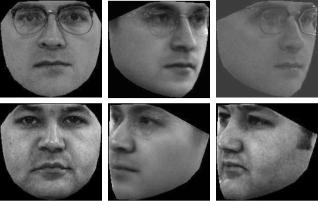
Fig. 9.2. Our eigen light-field estimation algorithm for re-rendering a face across pose. The algorithm is given the left-most (frontal) image as input from which it estimates the eigen light-field and then creates the rotated view shown in the middle. For comparison, the original rotated view is shown in the right-most column. In the figure we show one of the better results (top) and one of the worst (bottom.) Although in both cases the output looks like a face, the identity is altered in the second case.

where m and n range over their allowed values. (In general, the eigen light-fields Ei need to be interpolated to estimate Ei(θm,n, φm,n). Also, all of the equations for which the pixel I(m, n) does not image the object should be excluded from the computation.)

Although we have described this algorithm for a single image I(m, n), any number of images can obviously be used (so long as the camera intrinsics and relative orientation to the object are known for each image). The extra pixels from the other images are simply added in as additional constraints on the unknown coefficients λi in Eq. (3). The algorithm can be used to estimate a light-field from a collection of images. Once the light-field has been estimated, it can then be used to render new images of the same object under different poses. (See Vetter and Poggio [48] for a related algorithm.) We have shown [21] that the algorithm correctly re-renders a given object assuming a Lambertian reflectance model. The extent to which these assumptions are valid are illustrated in Figure 9.2, where we present the results of using our algorithm to re-render faces across pose. In each case the algorithm received the left-most (frontal) image as input and created the rotated view in the middle. For comparison, the original rotated view is included as the right-most image. The re-rendered image for the first subject is similar to the original. Although the image created for the second subject still shows a face in the correct pose, the identity of the subject is not as accurately recreated. We conclude that overall our algorithm works fairly well but that more training data are needed so the eigen light-field of faces can more accurately represent any given face light-field.

200 Ralph Gross, Simon Baker, Iain Matthews, and Takeo Kanade

Input Images		Classified Faces	Light−Field Vector
		L. Profile
		Left 3/4	Missing
	Classify by Pose	Frontal
			Normalize
		R. Profile	Missing

Fig. 9.3. Vectorization by normalization. Vectorization is the process of converting a set of images of a face into a light-field vector. Vectorization is performed by first classifying each input image into one of a finite number of poses. For each pose, normalization is then applied to convert the image into a subvector of the light-field vector. If poses are missing, the corresponding part of the light-field vector is missing.

2.2 Application to Face Recognition Across Pose

The eigen light-field estimation algorithm described above is somewhat abstract. To be able to use it for face recognition across pose we need to do the following things.

Vectorization: The input to a face recognition algorithm consists of a collection of images (possibly just one) captured from a variety of poses. The eigen light-field estimation Algorithm operates on light-field vectors (light-fields represented as vectors). Vectorization consists of converting the input images into a light-field vector (with missing elements, as appropriate.)

Classification: Given the eigen coefficients a1 . . . ad for a collection of gallery faces and for a probe face, we need to classify which gallery face is the most likely match.

Selecting training and testing sets: To evaluate our algorithm we have to divide the database used into (disjoint) subsets for training and testing.

We now describe each of these tasks in turn.

Vectorization by Normalization

Vectorization is the process of converting a collection of images of a face into a light-field vector. Before we can do this we first have to decide how to discretize the light-field into pixels. Perhaps the most natural way to do this is to uniformly sample the light-field angles (θ and φ in the 2D case of Figure 9.1). This is not the only way to discretize the light-field. Any sampling, uniform or nonuniform, could be used. All that is needed is a way to specify what is the allowed set of light-field pixels. For each such pixel, there is a corresponding index in the

Chapter 9. Face Recognition Across Pose and Illumination

201

light-field vector; that is, if the light-field is sampled at K pixels, the light-field vectors are K dimensional vectors.

We specify the set of light-field pixels in the following manner. We assume that there are only a finite set of poses 1, 2, . . . , P in which the face can occur. Each face image is first classified into the nearest pose. (Although this assumption is clearly an approximation, its validity is demonstrated by the empirical results in Section 2.3. In both the FERET [39] and PIE [46] databases, there is considerable variation in the pose of the faces. Although the subjects are asked to place their face in a fixed pose, they rarely do this perfectly. Both databases therefore contain considerable variation away from the finite set of poses. Our algorithm performs well on both databases, so the approximation of classifying faces into a finite set of poses is validated.)

Each pose i = 1, . . . , P is then allocated a fixed number of pixels Ki. The total number

of pixels in a light-field vector is therefore K =			P
			i=1 Ki. If we have images from poses 3
and 7, for example, we know K3 + K7 of the K	pixels in the light-field vector. The remaining

K −K3 −K7 are unknown, missing data. This vectorization process is illustrated in Figure 9.3. We still need to specify how to sample the Ki pixels of a face in pose i. This process is analogous to that needed in appearance-based object recognition and is usually performed by “normalization.” In eigenfaces [47], the standard approach is to find the positions of several canonical points, typically the eyes and the nose, and to warp the input image onto a coordinate frame where these points are in fixed locations. The resulting image is then masked. To generalize eigenface normalization to eigen light-fields, we just need to define such a normalization

for each pose.

We report results using two different normalizations. The first is a simple one based on the location of the eyes and the nose. Just as in eigenfaces, we assume that the eye and nose locations are known, warp the face into a coordinate frame in which these canonical points are in a fixed location, and finally crop the image with a (pose-dependent) mask to yield the Ki pixels. For this simple three-point normalization, the resulting masked images vary in size between 7200 and 12,600 pixels, depending on the pose.

The second normalization is more complex and is motivated by the success of active appearance models (AAMs) [12]. This normalization is based on the location of a large number (39–54 depending on the pose) of points on the face. These canonical points are triangulated and the image warped with a piecewise affine warp onto a coordinate frame in which the canonical points are in fixed locations. The resulting masked images for this multipoint normalization vary in size between 20,800 and 36,000 pixels. Although currently the multipoint normalization is performed using hand-marked points, it could be performed by fitting an AAM [12] and then using the implied canonical point locations.

Classification Using Nearest Neighbor

The eigen light-field estimation algorithm outputs a vector of eigen coefficients (a1, . . . , ad). Given a set of gallery faces, we obtain a corresponding set of vectors (aid1 , . . . , aidd ), where id is an index over the set of gallery faces. Similarly, given a probe face, we obtain a vector (a1, . . . , ad) of eigen coefficients for that face. To complete the face recognition algorithm we need an algorithm that classifies (a1, . . . , ad) with the index id, which is the most likely match. Many classification algorithms could be used for this task. For simplicity, we use the nearestneighbor algorithm, that classifies the vector (a1, . . . , ad) with the index.

202 Ralph Gross, Simon Baker, Iain Matthews, and Takeo Kanade

					d
		id	id		i		id		2
arg min dist		(a1, . . . , ad), (a1	, . . . , ad )	= arg	min	a	i − ai		(4)
id					id
					=1

All of the results reported in this chapter use the Euclidean distance in Eq. (4). Alternative distance functions, such as the Mahalanobis distance, could be used instead if so desired.

Selecting the Gallery, Probe, and Generic Training Data

In each of our experiments we divided the database into three disjoint subsets:

Generic training data: Many face recognition algorithms such as eigenfaces, and including our algorithm, require “generic training data” to build a generic face model. In eigenfaces, for example, generic training data are needed to compute the eigenspace. Similarly, in our algorithm, generic data are needed to construct the eigen light-field.

Gallery: The gallery is the set of reference images of the people to be recognized (i.e., the images given to the algorithm as examples of each person who might need to be recognized).

Probe: The probe set contains the “test” images (i.e., the images to be presented to the system to be classified with the identity of the person in the image).

The division into these three subsets is performed as follows. First we randomly select half of the subjects as the generic training data. The images of the remaining subjects are used for the gallery and probe. There is therefore never any overlap between the generic training data and the gallery and probe.

After the generic training data have been removed, the remainder of the databases are divided into probe and gallery sets based on the pose of the images. For example, we might set the gallery to be the frontal images and the probe set to be the left profiles. In this case, we evaluate how well our algorithm is able to recognize people from their profiles given that the algorithm has seen them only from the front. In the experiments described below we choose the gallery and probe poses in various ways. The gallery and probe are always disjoint unless otherwise noted.

2.3 Experimental Results

Databases

We used two databases in our face recognition across pose experiments, the CMU Pose, Illumination, and Expression (PIE) database [46] and the FERET database [39]. Each of these databases contains substantial pose variation. In the pose subset of the CMU PIE database (Fig. 9.4), the 68 subjects are imaged simultaneously under 13 poses totaling 884 images. In the FERET database, the subjects are imaged nonsimultaneously in nine poses. We used 200 subjects from the FERET pose subset, giving 1800 images in total. If not stated otherwise, we used half of the available subjects for training of the generic eigenspace (34 subjects for PIE, 100 subjects for FERET) and the remaining subjects for testing. In all experiments (if not stated otherwise) we retain a number of eigenvectors sufficient to explain 95% of the variance in the input data.

		Chapter 9. Face Recognition Across Pose and Illumination						203
c25			c09		c31
			0
0			(00 )		(−47	0	)
(44 )
				c27
c22	c02	c37	c05	c29	c11		c14	c34
(620)	(440)	(310)	(160)	(−170)	(−320)		(−460)	(−660 )
			c07
			(000)

Fig. 9.4. Pose variation in the PIE database. The pose varies from full left profile (c34) to full frontal (c27) and to full right profile (c22). Approximate pose angles are shown below the camera numbers.

Comparison with Other Algorithms

We compared our algorithm with eigenfaces [47] and FaceIt, the commercial face recognition system from Identix (formerly Visionics).1

We first performed a comparison using the PIE database. After randomly selecting the generic training data, we selected the gallery pose as one of the 13 PIE poses and the probe pose as any other of the remaining 12 PIE poses. For each disjoint pair of gallery and probe poses, we computed the average recognition rate over all subjects in the probe and gallery sets. The details of the results are shown in Figure 9.5 and are summarized in Table 9.1.

In Figure 9.5 we plotted color-coded 13 × 13 “confusion matrices” of the results. The row denotes the pose of the gallery, the column the pose of the probe, and the displayed intensity the average recognition rate. A lighter color denotes a higher recognition rate. (On the diagonals the gallery and probe images are the same so all three algorithms obtain a 100% recognition rate.)

Eigen light-fields performed far better than the other algorithms, as witnessed by the lighter color of Figure 9.5a,b compared to Figures 9.5c,d. Note how eigen light-fields was far better able to generalize across wide variations in pose, and in particular to and from near-profile views.

Table 9.1 includes the average recognition rate computed over all disjoint gallery-probe poses. As can be seen, eigen light-fields outperformed both the standard eigenfaces algorithm and the commercial FaceIt system.

We next performed a similar comparison using the FERET database [39]. Just as with the PIE database, we selected the gallery pose as one of the nine FERET poses and the probe pose as any other of the remaining eight FERET poses. For each disjoint pair of gallery and probe poses, we computed the average recognition rate over all subjects in the probe and gallery sets, and then averaged the results. The results are similar to those for the PIE database and are summarized in Table 9.2. Again, eigen light-fields performed significantly better than either FaceIt or eigenfaces.

Overall, the performance improvement of eigen light-fields over the other two algorithms is more significant on the PIE database than on the FERET database. This is because the PIE

1 Version 2.5.0.17 of the FaceIt recognition engine was used in the experiments.

204 Ralph Gross, Simon Baker, Iain Matthews, and Takeo Kanade

c22

c22

100

c02

c02

90

c25

c25

80

c37

c37

c05

c05

70

c07

c07

c27

c27

60

c09

c09

c29

c29

50

c11

c11

c14

c14

40

c31

c31

30

c34

c34

c22

c02

c25

c37

c05

c07

c27

c09

c29

c11

c14

c31

c34

c22

c02

c25

c37

c05

c07

c27

c09

c29

c11

c14

c31

c34

(a) Eigen Light-Fields - 3-Point Norm (b) Eigen Light-Fields - Multi-point Norm

c22

c22

100

90

c02

c02

c25

c25

80

c37

c37

70

c05

c05

c07

c07

60

c27

c27

50

c09

c09

c29

c29

40

c11

c11

30

c14

c14

20

c31

c31

c34

c34

10

c22

c02

c25

c37

c05

c07

c27

c09

c29

c11

c14

c31

c34

c22

c02

c25

c37

c05

c07

c27

c09

c29

c11

c14

c31

c34

(c) FaceIt

(d) eigenfaces

Fig. 9.5. Comparison with FaceIt and eigenfaces for face recognition across pose on the CMU PIE [46] database. For each pair of gallery and probe poses, we plotted the color-coded average recognition rate. The row denotes the pose of the gallery and the column the pose of the probe. The fact that the images in a and b are lighter in color than those in c and d implies that our algorithm performs better.

database contains more variation in pose than the FERET database. For more evaluation results see Gross et al. [23].

Table 9.1. Comparison of eigen light-fields with FaceIt and eigenfaces for face recognition across pose on the CMU PIE database. The table contains the average recognition rate computed across all disjoint pairs of gallery and probe poses; it summarizes the average performance in Figure 9.5.

Algorithm	Average recognition accuracy (%)
Eigenfaces	16.6
FaceIt	24.3
Eigen light-fields
Three-point norm	52.5
Multipoint norm	66.3

Chapter 9. Face Recognition Across Pose and Illumination

205

Table 9.2. Comparison of eigen light-fields with FaceIt and eigenfaces for face recognition across pose on the FERET database. The table contains the average recognition rate computed across all disjoint pairs of gallery and probe poses. Again, eigen light-fields outperforms both eigenfaces and FaceIt.

Algorithm	Average recognition accuracy (%)
Eigenfaces	39.4
FaceIt	59.3
Eigen light-fields three-point normalization	75.0

3 Bayesian Face Subregions

Owing to the complicated 3D nature of the face, differences exist in how the appearance of various face regions change for different face poses. If, for example, a head rotates from a frontal to a right profile position, the appearance of the mostly featureless cheek region only changes little (if we ignore the influence of illumination), while other regions such as the left eye disappear, and the nose looks vastly different. Our algorithm models the appearance changes of the different face regions in a probabilistic framework [28]. Using probability distributions for similarity values of face subregions; we compute the likelihood of probe and gallery images coming from the same subject. For training and testing of our algorithm we use the CMU PIE database [46].

3.1 Face Subregions and Feature Representation

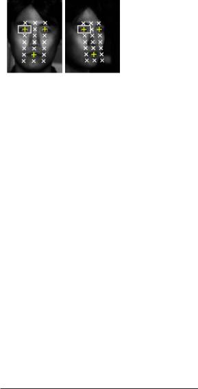
Using the hand-marked locations of both eyes and the midpoint of the mouth, we warp the input face images into a common coordinate frame in which the landmark points are in a fixed location and crop the face region to a standard 128 × 128 pixel size. Each image I in the database is labeled with the identity i and pose φ of the face in the image: I = (i, φ), i {1, . . . , 68}, φ {1, . . . , 13}. As shown in Figure 9.6, a 7 × 3 lattice is placed on the normalized faces, and 9 × 15 pixel subregions are extracted around every lattice point. The intensity values in each of the 21 subregions are normalized to have zero mean and unit variance.

As the similarity measure between subregions we use SSD (sum of squared difference) values sj between corresponding regions j for all image pairs. Because we compute the SSD after image normalization, it effectively contains the same information as normalized correlation.

3.2 Modeling Local Appearance Change Across Pose
For probe image Ii,p =				(i, φp) with unknown identity i we compute the probability that
Ii,p is coming from the same subject k as gallery image Ik,g for each face subregion j, j
{1, . . . , 21}. Using Bayes’ rule we write:
P (i = k s	, φ , φ		) =	P (sj |i = k, φp, φg )P (i = k)	(5)
				P (sj |i = k, φp, φg )P (i = k) + P (sj |i =k, φp, φg )P (i =k)
| j	p	g

206 Ralph Gross, Simon Baker, Iain Matthews, and Takeo Kanade

Fig. 9.6. Face subregions for two poses of the CMU PIE database. Each face in the database is warped into a normalized coordinate frame using the hand-labeled locations of both eyes and the midpoint of the mouth. A 7 × 3 lattice is placed on the normalized face, and 9 × 15 pixel subregions are extracted around every lattice point, resulting in a total of 21 subregions.

We assume the conditional probabilities P (sj |i = k, φp, φg ) and P (sj |i =k, φp, φg ) to be Gaussian distributed and learn the parameters from data. Figure 9.7 shows histograms of similarity values for the right eye region. The examples in Figure 9.7 show that the discriminative power of the right eye region diminishes as the probe pose changes from almost frontal (Figure 9.7a) to right profile (Figure 9.7c).

It is reasonable to assume that the pose of each gallery image is known. However, because the pose φp of the probe images is in general not known, we marginalize over it. We can then compute the conditional densities for similarity value sj as

P (sj |i = k, φg ) = P (φp)P (sj |i = k, φp, φg )

p

and

P (sj |i =k, φg ) = P (φp)P (sj |i =k, φp, φg )

p

If no other knowledge about the probe pose is given, the pose prior P (φp) is assumed to be uniformly distributed. Similar to the posterior probability defined in Eq. (5) we compute the probability of the unknown probe image coming from the same subject (given similarity value sj and gallery pose φg ) as

	P (i = k s	, φ ) =	P (sj |i = k, φg )P (i = k)	(6)
			P (sj |i = k, φg )P (i = k) + P (sj |i =k, φg )P (i =k)
	| j	g

To decide on the most likely identity of an unknown probe image Ii,p = (i, φp) we compute match probabilities between Ii,p and all gallery images for all face subregions using Eq. (5) or (6). We currently do not model dependencies between subregions, so we simply combine the different probabilities using the sum rule [29] and choose the identity of the gallery image with the highest score as the recognition result.

Chapter 9. Face Recognition Across Pose and Illumination

207

(a) c27 vs. c5

(b) c27 vs. c37

(c) c27 vs. c22

Fig. 9.7. Histograms of similarity values sj for the right eye region across multiple poses. The distribution of similarity values for identical gallery and probe subjects are shown with solid curves, the distributions for different gallery and probe subjects are shown with broken curves.

3.3 Experimental Results

We used half of the 68 subjects in the CMU PIE database for training of the models described in Section 3.2. The remaining 34 subjects are used for testing. The images of all 68 subjects are used in the gallery. We compare our algorithm to eigenfaces [47] and the commercial FaceIt system.

Experiment 1: Unknown Probe Pose

For the first experiment we assume the pose of the probe images to be unknown. We therefore must use Eq. (6) to compute the posterior probability that probe and gallery images come from the same subject. We assume P (φp) to be uniformly distributed, that is, P (φp) = 131 . Figure 9.8 compares the recognition accuracies of our algorithm with eigenfaces and FaceIt for frontal gallery images. Our system clearly outperforms both eigenfaces and FaceIt. Our algorithm shows good performance up until 45◦ head rotation between probe and gallery image (poses 02 and 31). The performance of eigenfaces and FaceIt already drops at 15◦ and 30◦ rotation, respectively.

Experiment 2: Known Probe Pose

In the case of known probe pose we can use Eq. (5) to compute the probability that probe and gallery images come from the same subject. Figure 9.9 compares the recognition accuracies of our algorithm for frontal gallery images for known and unknown probe poses. Only small differences in performances are visible.

208 Ralph Gross, Simon Baker, Iain Matthews, and Takeo Kanade

											BFS
											FaceIt
											EigenFace
	100
Correct	80
Percent	60
	40
	20
	0	31	14	11	29	09	27	07	05	37	25	02	22
	34
						Probe Pose

Fig. 9.8. Recognition accuracies for our algorithm (labeled BFS), eigenfaces, and FaceIt for frontal gallery images and unknown probe poses. Our algorithm clearly outperforms both eigenfaces and FaceIt.

										Known case
										Unknown case
	100
Correct	80
Percent	60
	40
	20
	0	31	14	11	29	09	27	07	05	37	25	02	22
	34
						Probe Pose

Fig. 9.9. Comparison of recognition accuracies of our algorithm for frontal gallery images for known and unknown probe poses. Only small differences are visible.

Figure 9.10 shows recognition accuracies for all three algorithms for all possible combinations of gallery and probe poses. The area around the diagonal in which good performance is achieved is much wider for our algorithm than for either eigenfaces or FaceIt. We therefore conclude that our algorithm generalizes much better across pose than either eigenfaces or FaceIt.

Chapter 9. Face Recognition Across Pose and Illumination

209

(a) Our algorithm

(b) Eigenfaces

(c) FaceIt

Fig. 9.10. Recognition accuracies for our algorithm, eigenfaces, and FaceIt for all possible combinations of gallery and probe poses. Here lighter pixel values correspond to higher recognition accuracies. The area around the diagonal in which good performance is achieved is much wider for our algorithm than for either eigenfaces or FaceIt.

4 Face Recognition Across Pose and Illumination

Because appearance-based methods use image intensities directly, they are inherently sensitive to variations in illumination. Drastic changes in illumination such as between indoor and outdoor scenes therefore cause significant problems for appearance-based face recognition algorithms [24, 38]. In this section we describe two ways to handle illumination variations in facial imagery. The first algorithm extracts illumination invariant subspaces by extending the previously introduced eigen light-fields to Fisher light-fields [22], mirroring the step from eigenfaces [47] to fisherfaces [4]. The second approach combines Bayesian face subregions with an image preprocessing algorithm that removes illumination variation prior to recognition [20]. In both cases we demonstrate results for face recognition across pose and illumination.

4.1 Fisher Light-Fields

Suppose we are given a set of light-fields Li,j (θ, φ), i = 1, . . . , N, j = 1, . . . , M where each of N objects Oi is imaged under M different illumination conditions. We could proceed as described in Section 2.1 and perform PCA on the whole set of N ×M light-fields. An alternative approach is Fisher’s linear discriminant (FLD) [14], also known as linear discriminant analysis (LDA) [51], which uses the available class information to compute a projection better suited for discrimination tasks. Analogous to the algorithm described in Section 2.1, we now find the least-squares solution to the set of equations

m
i	λiWi(θ, φ) = 0	(7)
L(θ, φ) −
=1

where Wi, i = 1, . . . , m are the generalized eigenvectors computed by LDA.

210 Ralph Gross, Simon Baker, Iain Matthews, and Takeo Kanade

Table 9.3. Performance of eigen light-fields and Fisher light-fields with FaceIt on three face recognition across pose and illumination scenarios. In all three cases, eigen light-fields and Fisher light-fields outperformed FaceIt by a large margin.

Conditions	Eigen light-fields	Fisher light-fields	FaceIt
Same pose, different illumination	-	81.1%	41.6%
Different pose, same illumination	72.9%	-	25.8%
Different pose, different illumination	-	36.0%	18.1%

Experimental Results

For our face recognition across pose and illumination experiments we used the pose and illumination subset of the CMU PIE database [46]. In this subset, 68 subjects are imaged under 13 poses and 21 illumination conditions. Many of the illumination directions introduce fairly subtle variations in appearance, so we selected 12 of the 21 illumination conditions that span the set widely. In total we used 68 × 13 × 12 = 10, 608 images in the experiments.

We randomly selected 34 subjects of the PIE database for the generic training data and then removed the data from the experiments (see Section 2.2). There were then a variety of ways to select the gallery and probe images from the remaining data.

Same pose, different illumination: The gallery and probe poses are the same. The gallery and probe illuminations are different. This scenario is like traditional face recognition across illumination but is performed separately for each pose.

Different pose, same illumination: The gallery and probe poses are different. The gallery and probe illuminations are the same. This scenario is like traditional face recognition across pose but is performed separately for each possible illumination.

Different pose, different illumination: Both the pose and illumination of the probe and gallery are different. This is the most difficult and most general scenario.

We compared our algorithms with FaceIt under these three scenarios. In all cases we generated every possible test scenario and then averaged the results. For “same pose, different illumination,” for example, we consider every possible pose. We generated every pair of disjoint probe and gallery illumination conditions. We then computed the average recognition rate for each such case. We averaged over every pose and every pair of distinct illumination conditions. The results are included in Table 9.3. For “same-pose, different illumination,” the task is essentially face recognition across illumination separately for each pose. In this case, it makes little sense to try eigen light-fields because we know how poorly eigenfaces performs with illumination variation. Fisher light-fields becomes fisherfaces for each pose, which empirically we found outperforms FaceIt. Example illumination “confusion matrices” are included for two poses in Figure 9.11.

For “different pose, same illumination,” the task reduces to face recognition across pose but for a variety of illumination conditions. In this case there is no intraclass variation, so it makes little sense to apply Fisher light-fields. This experiment is the same as Experiment 1 in Section 2.3 but the results are averaged over every possible illumination condition. As we found for Experiment 1, eigen light-fields outperforms FaceIt by a large amount.

Chapter 9. Face Recognition Across Pose and Illumination

211

Probe Flash Conditions

f16

f15

f13

f21

f12

f11

f08

f06

f10

f18

f04

f02

f16

f15

f13

Conditions f11

f21

f12

Flash

f08

Probe f10

f06

f18

f04

f02

f16

f15

f13

f21

f12

f11

f08

f06

f10

f18

f04

f02

f16

f15

f13

f21

f12

f11

f08

f06

f10

f18

f04

f02

Gallery Flash Conditions

Gallery Flash Conditions

100

90

80

70

60

50

40

(a) Fisher LF - Pose c27 vs. c27 (frontal)

(c) FaceIt - Pose c27 vs. c27

f16

f16

f15

f15

Conditions

f13

Conditions

f13

f11

f11

f21

f21

f12

f12

Flash

f08

Flash

f08

Probe

f10

Probe

f10

f06

f06

f18

f18

f04

f04

f02

f02

f16

f15

f13

f21

f12

f11

f08

f06

f10

f18

f04

f02

f16

f15

f13

f21

f12

f11

f08

f06

f10

f18

f04

f02

Gallery Flash Conditions

Gallery Flash Conditions

(b) Fisher LF - Pose c37 vs. c37 (right 3/4)

(d) FaceIt - Pose c37 vs. c37

100

90

80

70

60

50

40

30

20

10

0

Fig. 9.11. Example “confusion matrices” for the “same-pose, different illumination” task. For a given pose, and a pair of distinct probe and gallery illumination conditions, we color-code the average recognition rate. The superior performance of Fisher light-fields is witnessed by the lighter color of (a–b) over (c–d).

Finally, in the “different pose, different illumination” task both algorithms perform fairly poorly. However, the task is difficult. If the pose and illumination are both extreme, almost none of the face is visible. Because this case might occur in either the probe or the gallery, the chance that such a difficult case occurs is large. Although more work is needed on this task, note that Fisher light-fields still outperforms FaceIt by a large amount.

4.2 Illumination Invariant Bayesian Face Subregions

In general, an image I(x, y) is regarded as product I(x, y) = R(x, y)L(x, y), where R(x, y) is the reflectance and L(x, y) is the illuminance at each point (x, y) [26]. Computing the reflectance and the illuminance fields from real images is, in general, an ill-posed problem. Our approach uses two widely accepted assumptions about human vision to solve the problem: (1) human vision is mostly sensitive to scene reflectance and mostly insensitive to the illumination conditions; and (2) human vision responds to local changes in contrast rather than to global brightness levels. Our algorithm computes an estimate of L(x, y) such that when it divides I(x, y) it produces R(x, y) in which the local contrast is appropriately enhanced. We find a

212 Ralph Gross, Simon Baker, Iain Matthews, and Takeo Kanade

Original PIE images

Processed PIE images

Fig. 9.12. Result of removing illumination variations with our algorithm for a set of images from the PIE database.

solution for L(x, y) by minimizing
J(L) = Ω ρ(x, y)(L − I)2dxdy + λ Ω (Lx2 + Ly2 )dxdy	(8)

Here Ω refers to the image. The parameter λ controls the relative importance of the two terms. The space varying permeability weight ρ(x, y) controls the anisotropic nature of the smoothing constraint. See Gross and Brajovic [20] for details. Figure 9.12 shows examples from the CMU PIE database before and after processing with our algorithm. We used this algorithm to normalize the images of the combined pose and illumination subset of the PIE database. Figure 9.13 compares the recognition accuracies of the Bayesian face subregions algorithm for original and normalized images using gallery images with frontal pose and illumination. The algorithm achieved better performance on normalized images across all probe poses. Overall the average recognition accuracy improved from 37.3% to 44%.

5 Conclusions

One of the most successful and well studied approaches to object recognition is the appearancebased approach. The defining characteristic of appearance-based algorithms is that they directly use the pixel intensity values in an image of the object as the features on which to base the recognition decision. In this chapter we described an appearance-based method for face recognition across pose based on an algorithm to estimate the eigen light-field from a collection of images. Unlike previous appearance-based methods, our algorithm can use any number of gallery images captured from arbitrary poses and any number of probe images also captured from arbitrary poses. The gallery and probe poses do not need to overlap. We showed that our

Chapter 9. Face Recognition Across Pose and Illumination

213

100

Original

90

Normalized

80

70

[%]

60

Accuracy

50

40

30

20

10

0

c02

c25

c37

c05

c07

c27

c09

c29

c11

c14

c31

c34

c22

Probe Pose

Fig. 9.13. Recognition accuracies of the Bayesian face subregions algorithm on original and normalized images using gallery images with frontal pose and illumination. For each probe pose the accuracy is determined by averaging the results for all 21 illumination conditions. The algorithm achieves better performance on normalized images across all probe poses. The probe pose is assumed to be known.

algorithm can reliably recognize faces across pose and also take advantage of the additional information contained in widely separated views to improve recognition performance if more than one gallery or probe image is available.

In eigen light-fields all face pixels are treated equally. However, differences exist in how the appearance of various face regions change across face poses. We described a second algorithm, Bayesian face subregions, which derives a model for these differences and successfully employes it for face recognition across pose. Finally, we demonstrated how to extend both algorithms toward face recognition across both pose and illumination. Note, however, that for this task recognition accuracies are significantly lower, suggesting that there still is room for improvement. For example, the model-based approach of Romdhani et al.[40] achieved better results across pose on the PIE database than the appearance-based algorithms described here.

Acknowledgments

The research described here was supported by U.S. Office of Naval Research contract N00014- 00-1-0915 and in part by U.S. Department of Defense contract N41756-03-C4024. Portions of the research in this paper used the FERET database of facial images collected under the FERET program.

214 Ralph Gross, Simon Baker, Iain Matthews, and Takeo Kanade

References

1.E. Adelson and J. Bergen. The plenoptic function and elements of early vision. In Landy and Movshon, editors, Computational Models of Visual Processing. MIT Press, Cambridge, MA, 1991.

2.Y. Adini, Y. Moses, and S. Ullman. Face recognition: The problem of compensating for changes in illumination direction. IEEE Transactions on Pattern Analysis and Machine Intelligence, 19(7):721– 732, 1997.

3.R. Basri and D. Jacobs. Lambertian reflectance and linear subspaces. IEEE Transactions on Pattern Analysis and Machine Intelligence, 25(2):218–233, 2003.

4.P. Belhumeur, J. Hespanha, and D. Kriegman. Eigenfaces vs. fisherfaces: recognition using class specific linear projection. IEEE Transactions on Pattern Analysis and Machine Intelligence, 19(7):711– 720, 1997.

5.P. Belhumeur and D. Kriegman. What is the set of images of an object under all possible lighting conditions. Int. J. of Computer Vision, 28(3):245–260, 1998.

6.D. Beymer. Face recognition under varying pose. Technical Report 1461, MIT AI Laboratory, Cambridge, MA, 1993.

7.D. Beymer and T. Poggio. Face recognition from one example view. A.I. Memo No. 1536, MIT AI Laboratory, Cambridge, MA, 1995.

8.M. Black and A. Jepson. Eigen-tracking: robust matching and tracking of articulated objects using a view-based representation. International Journal of Computer Vision, 36(2):101–130, 1998.

9.D. Blackburn, M. Bone, and P. Phillips. Facial recognition vendor test 2000: evaluation report, 2000.

10.V. Blanz and T. Vetter. Face recognition based on fitting a 3D morphable model. IEEE Transactions on Pattern Analysis and Machine Intelligence, 25(9):1063–1074, 2003.

11.V. Blanz, S. Romdhani, and T. Vetter. Face identification across different poses and illumination with a 3D morphable model. In Proceedings of the Fifth International Conference on Face and Gesture Recognition, pages 202–207, 2002.

12.T. Cootes, G. Edwards, and C. Taylor. Active appearance models. IEEE Transactions on Pattern Analysis and Machine Intelligence, 23(6):681–685, 2001.

13.T. Cootes, G. Wheeler, K. Walker, and C. Taylor. View-based active appearance models. Image and Vision Computing, 20:657–664, 2002.

14.K. Fukunaga. Introduction to Statistical Pattern Recognition. Academic Press, San Diego, CA, 1990.

15.A. Georghiades, P. Belhumeur, and D. Kriegman. From few to many: Generative models for recognition under variable pose and illumination. In Proceedings of the Fourth International Conference on Face and Gesture Recognition, pages 277–284, 2000.

16.A. Georghiades, D. Kriegman, and P. Belhumeur. Illumination cones for recognition under variable lighting: faces. In Proceedings of the IEEE Conference on Computer Vision and Pattern Recognition, 1998.

17.A. Georghiades, D. Kriegman, and P. Belhumeur. From few to many: generative models for recognition under variable pose and illumination. IEEE Transactions on Pattern Analysis and Machine Intelligence, 23(6):643–660, 2001.

18.S. Gortler, R. Grzeszczuk, R. Szeliski, and M. Cohen. The lumigraph. In Computer Graphics Proceedings, Annual Conference Series (SIGGRAPH), pages 43–54, 1996.

19.D. Graham and N. Allison. Face recognition from unfamiliar views: subspace methods and pose dependency. In 3rd International Conference on Automatic Face and Gesture Recognition, pages 348–353, 1998.

20.R. Gross and V. Brajovic. An image pre-processing algorithm for illumination invariant face recognition. In 4th International Conference on Audioand Video Based Biometric Person Authentication (AVBPA), pages 10–18, June 2003.

21.R. Gross, I. Matthews, and S. Baker. Eigen light-fields and face recognition across pose. In Proceedings of the Fifth International Conference on Face and Gesture Recognition, pages 1–7, 2002.

Chapter 9. Face Recognition Across Pose and Illumination

215

22.R. Gross, I. Matthews, and S. Baker. Fisher light-fields for face recognition across pose and illumination. In Proceedings of the German Symposium on Pattern Recognition (DAGM), pages 481–489, 2002.

23.R. Gross, I. Matthews, and S. Baker. Appearance-based face recognition and light-fields. IEEE Transactions on Pattern Analysis and Machine Intelligence, 26(4):449–465, 2004.

24.R. Gross, J. Shi, and J. Cohn. Quo vadis face recognition? In Third Workshop on Empirical Evaluation Methods in Computer Vision, 2001.

25.B. Horn. Determining lightness from an image. Computer Graphics and Image Processing, 3(1):277– 299, 1974.

26.B. Horn. Robot Vision. MIT Press, Cambridge, MA, 1986.

27.D. Jacobs, P. Belhumeur, and R. Basri. Comparing images under variable illumination. In IEEE Conference on Computer Vision and Pattern Recognition, pages 610–617, 1998.

28.T. Kanade and A. Yamada. Multi-subregion based probabilistic approach toward pose-invariant face recognition. In IEEE International Symposium on Computational Intelligence in Robotics and Automation (CIRA2003), pages 954–959, 2003.

29.J. Kittler, M. Hatef, R. Duin, and J. Matas. On combining classifiers. IEEE Trans. on Pattern Analysis and Machine Intelligence, 20(3):226–239, 1998.

30.E. Land and J. McCann. Lightness and retinex theory. Journal of the Optical Society of America, 61(1):1–11, 1971.

31.M. Lando and S. Edelman. Generalization from a single view in face recognition. In International Workshop on Automatic Face-and Gesture-Recognition, 1995.

32.A. Lanitis, C. Taylor, and T. Cootes. Automatic interpretation and coding of face images using flexible models. IEEE Transactions on Pattern Analysis and Machine Intelligence, 19(7):743–756, 1997.

33.A. Leonardis and H. Bischof. Robust recognition using eigenimages. Computer Vision and Image Understanding, 78(1):99–118, 2000.

34.M. Levoy and M. Hanrahan. Light field rendering. In Computer Graphics Proceedings, Annual Conference Series (SIGGRAPH), pages 31–41, 1996.

35.T. Maurer and C. von der Malsburg. Single-view based recognition of faces rotated in depth. In

International Workshop on Automatic Face and Gesture Recogition, pages 248–253, 1995.

36.H. Murase and S. Nayar. Visual learning and recognition of 3-D objects from appearance. International Journal of Computer Vision, 14:5–24, 1995.

37.A. Pentland, B. Moghaddam, and T. Starner. View-based and modular eigenspaces for face recognition. In Proceedings of the IEEE Conference on Computer Vision and Pattern Recognition, pages 84–91, 1994.

38.P. J. Phillips, P. Grother, J. Ross, D. Blackburn, E. Tabassi, and M. Bone. Face recognition vendor test 2002: evaluation report, March 2003.

39.P. J. Phillips, H. Moon, S. Rizvi, and P. Rauss. The FERET evaluation methodology for face-recognition algorithms. IEEE Transactions on Pattern Analysis and Machine Intelligence, 22(10):1090–1104, 2000.

40.S. Romdhani, V. Blanz, and T. Vetter. Face identification by matching a 3D morphable model using linear shape and texture error functions. In Proceedings of the European Conference on Computer Vision, pages 3–19, 2002.

41.S. Romdhani, S. Gong, and A. Psarrou. Multi-view nonlinear active shape model using kernel PCA. In 10th British Machine Vision Conference, volume 2, pages 483–492, 1999.

42.S. Romdhani, A. Psarrou, and S. Gong. On utilising template and feature-based correspondence in multi-view appearance models. In 6th European Conference on Computer Vision, volume 1, pages 799–813, 2000.

43.A. Shashua. Geometry and Photometry in 3D visual recognition. PhD thesis, MIT, 1994.

44.A. Shashua and T. Riklin-Raviv. The Quotient image: class-based re-rendering and recognition with varying illumination conditions. IEEE Transactions on Pattern Analysis and Machine Intelligence, 23(2):129–139, 2001.

216 Ralph Gross, Simon Baker, Iain Matthews, and Takeo Kanade

45.T. Sim and T. Kanade. Combining models and exemplars for face recognition: an illuminating example. In Workshop on Models versus Exemplars in Computer Vision, 2001.

46.T. Sim, S. Baker, and M. Bsat. The CMU pose, illumination, and expression database. IEEE Transactions on Pattern Analysis and Machine Intelligence, 25(12):1615–1618, 2003.

47.M. Turk and A. Pentland. Face recognition using eigenfaces. In Proceedings of the IEEE Conference on Computer Vision and Pattern Recognition, 1991.

48.T. Vetter and T. Poggio. Linear object classes and image synthesis from a single example image.

IEEE Transactions on Pattern Analysis and Machine Intelligence, 19(7):733–741, 1997.

49.L. Wiskott, J. Fellous, N. Kruger, and C. von der Malsburg. Face recognition by elastic bunch graph matching. IEEE Transactions on Pattern Analysis and Machine Intelligence, 19(7):775–779, 1997.

50.W. Zhao and R. Chellappa. Robust face recognition using symmetric shape-from-shading. Technical report, Center for Automation Research, University of Maryland, 1999.

51.W. Zhao, A. Krishnaswamy, R. Chellappa, D. Swets, and J. Weng. Discriminant analysis of principal components for face recognition. In H. Wechsler, P. J. Phillips, V. Bruce, and T. Huang, editors, Face Recognition: From Theory to Applications. Springer, New York, 1998.