Определение на фотографиях контуров лица и подбородка / !!!A Bayesian Model for Extracting Facial Features

A Bayesian Model for Extracting Facial Features

Zhong Xued, Stan Z. Li1, Juwei Lun, Eam Khwang Teohd

dSchool of EEE, Nanyang Technological University, Singapore 639798 1Microsoft Research China, No.49 Zhichun Road, Beijing 100080, China

nCenter for Signal Processing, Nanyang Technological University, Singapore 639798

Abstract

A Bayesian Model (BM) is proposed in this paper for extracting facial features. In the BM, first the prior distribution of object shapes, which reflects the global shape variations of the object contour, is estimated from the sample data. This distribution is then utilized to constrain and dynamically adjust the prototype contour in the matching procedure, in this way large or global shape deformations due to the variations of samples can be tolerated. Moreover, a transformational invariant internal energy term is introduced to describe mainly the local shape deformations between the prototype contour in the shape domain and the deformable contour in the image domain, so that the proposed BM can match the objects undergoing not only global but also local variations. Experiment results based on real facial feature extraction demonstrate that the BM is more robust and insensitive to the positions, viewpoints, and deformations of object shapes, as compared to the Active Shape Model (ASM) algorithm.

Keywords: Bayesian model (BM), deformable model, active shape model (ASM), object matching.

1 Introduction

Compared with traditional rigid models, deformable models have attracted much attention in the areas of object detection and matching because of their ability of adapting themselves to fit objects more closely. Generally, deformable models can be classified into two classes [1]: the free-form models and the parametric models. The free-form models, e.g. active contours or snakes, can be used to match any arbitrary shape provided some general regularization constraints, such as continuity and smoothness, are satisfied. On the other hand, the parametric models are more constrained because some prior information of the geometrical shape is incorporated. It has been demonstrated that the parametric models are more robust to irrelevant structures and occlusions when being applied to detect specific shapes of interest.

The parametric models, such as deformable tem-

plates/models [1] [2] [3] [4], G-Snake [5] and ASM [6], encode specific characteristics of a shape and its variations using global shape model, which is formed by a set of feature parameters or well defined landmark/boundary points of that shape. A quite successful and versatile scheme in this field is statistics-based shape models in Bayesian framework [1][5]. In these models, the prior knowledge of the object as well as the observation statistics is utilized to define the optimal Bayesian estimate. However, most of these existing parametric models encode the shape information in a “hard” manner in that the prototype contour is fixed during the matching process. As a result, only a small amount of local deformations can be tolerated.

The Active Shape Model (ASM) encodes the prior information of object shapes using principal component analysis (PCA), and matches object by directly using the geometrical transformed version of the ASM model. In ASM, the prototype used to match object can be dynamically adjusted in the matching procedure, which is constrained by the prior distribution of sample data. Therefore, some global/large shape variations that present in the sample data, can be tolerated. Recently, Cootes et. al. proposed an Active Appearance Model (AAM) [7], which contains a statistical model of the shape and greylevel appearance of an object of interest. The object matching is accomplished by measuring the current residuals and using the linear predict model learnt in the training phase. By combining the prior information of object shape and appearance, AAM can match object more effectively than ASM.

However, as a statistical model, ASM/AAM takes the reconstructed object model that matches the image best as the results of object matching. Therefore, it may not be able to match accurately to a new image if the variations of shape and appearance does not present in the sample data, or if the number of model modes has been truncated too severely. To match a new object more accurately, new methods should be proposed to deal with not only the global deformations defined by the model, but also the local random variations. In [8], the AAM is combined with a local model, i.e. during the matching procedure, the further local model deformations (the local AAMs) for each point are performed after the convergence of AAM, and a multi-resolution framework is also

used to enlarge the searching range of the model. Such a process can fit more accurately to unseen data than models using purely global model modes (ASM/ASM) or purely local models (Snakes). However, it has to build and train the local models for each point, which leads the shortcomings: more parameters are required to describe the model state; heavy computational load; it is difficult to judge the change between global AAM and local AAMs during the matching procedure.

In this paper, a Bayesian Model (BM), which serves as a framework to solve the global and local deformations in object matching, is proposed. In the BM, the prior distribution of object shapes and/or appearance, which reflects the global shape variations of the object, is estimated from the sample data. In the matching procedure, this prior distribution is used to constrain the dynamically adjustable prototype. In this way, large shape and/or appearance deformations due to the variations of samples can be tolerated. Moreover, since the shapes are subjected to some transformations between the shape space and the image space, such as similarity transformation and affine transformations, it is expected that the algorithms developed should be able to deal with the rotation, translation, scaling and even shearing. Therefore, a transformational invariant internal energy term is introduced in the BM to describe mainly the local shape deformations between the prototype contour in the shape domain and the deformable contour in the image domain. Because the deformable contour used to match object has been modeled as the transformed and deformed version of the prototype contour, which can also be dynamically adjusted to adapt itself to the shape variations using the information gathered from the matching process, the proposed BM has the advantage of matching objects with both global and local variations. Experiment results based on real facial feature extraction demonstrate that the BM is more accurate as compared to the Active Shape Model (ASM).

The rest of the paper is organized as follows: Section 2 introduces the BM, Section 3 describes the algorithm for facial feature extraction using BM and presents the experimental results, and Section 4 summarizes the conclusion from this study.

2 Bayesian Model (BM)

2.1Bayesian Framework and Energy Terms

The Bayesian Model (BM) formulates the matching of a deformable model to the object in a given image as a maximizing a posteriori (MAP) estimation problem. Denote the mean of the sample contours in the shape domain as Wƒ( (the mean contour), the deformed version

of Wƒ( as Wƒ (the prototype contour), and the deformable contour in the image domain as W, where Wƒ( ; p1 ] , Wƒ ; p1 ] and W ; p1 ] are the matrices representing the corresponding contours formed by the coordinates of ] landmark/boundary points. According to the Bayesian estimation, the joint posterior distribution of W and Wƒ,

€wW, Wƒ/QD, is

€wW, Wƒ/QD )	€wQ/WD€wW, WƒD	(1)
	€wQD

where €wQ/WD ) €wQ/W, WƒD is the likelihood distribution of input image data Q.

€wW, WƒD ) €wW/WƒD€wWƒD

(2)

is the joint prior distribution of W and Wƒ.

For a given image Q, the MAP estimates, W-\h and Wƒ-\h , can be defined as,

\W-\h , Wƒ-\h i ) s„ 8s- \€wW, Wƒ/QDi
	W,Wƒ
) s„ 8s- \	€wQ/WD€wW/WƒD€wWƒD i	(3)
W,Wƒ	€wQD

where €wWƒD is the distribution of the prototype Wƒ, €wW/WƒD describes the variations between W and Wƒ, and €wQ/WD indicates the matching between W and the salient features of the object in image Q. It can be seen from Eq.3 that BM estimates the suitable prototype shape Wƒ, and obtains a best deformable contour in the image domain W to match the object. Therefore, in the BM, not only the prototype, but also the deformation between W and the prototype Wƒ can be adaptively adjustable.

Provided the densities in Eq. (3) can be modeled as Gibb’s distribution, i.e.

€wWƒD	)	.d d ‚-} \ o•LzwWƒDi
€wW/WƒD	)	d ‚-} \ o	7z0	wW/WƒDi	(4)
		.1

€wQ/WD ) .n d ‚-} \ o ?0wQ/WDi

where .d, .1 and .n are the partition functions, maximizing the posterior distribution is equivalent to minimizing the corresponding energy function of the contour:

\W-\h , Wƒ-\h i ) s„ 8$t \o•Lz0L`„i

(5)

ƒ

W,W

where o•Lz0L`„ ) o•Lz Lo7z0 Lo ?0. o•Lz ) o•LzwWƒD

is the constraint energy term of the adjustable prototype contour Wƒ, which limits the variations of Wƒ and ensures that Wƒ is similar with Wƒ( in shape. Wƒ( is the mean of all the aligned sample contours in the shape domain. o7z0 ) o7z0wW/WƒD is the internal energy term that describes the global and local shape deformation between W and Wƒ. The external energy term o ?0 ) o ?0wQ/WD defines the degree of matching between W and the salient features of image Q.

2.2The Constraint Energy of Prototype

The constraint energy term o•Lz of the prototype contour is caused by the prior distribution, €wWƒD, of the samples in the shape domain, which can be estimated from the normalized sample data and reflects the shape variations of the shapes in the shape domain. Linear or nonlinear methods can be used to estimate this prior distribution according to the application. In this paper, the method using PCA to estimate €wWƒD is utilized, which reflects mainly the linear relationship of the shape variations. In cases where all the samples are aligned views of similar objects seen from a standard view, this distribution can be accurately modeled by a single Gaussian distribution [9].

	d	-	j
€wWƒD )	‚-}w 1			D
		7)d			(6)
			db1
		-
	w1$D-b1 >)d >
where
j ) x wWƒ Wƒ(D					(7)
-

is the vector of the shape parameters, and Wƒ Wƒ( is the deformation from Wƒ( to Wƒ. - is the matrix composed of the eigenvectors corresponding to the largest - eigenvalues 7, wd 7 -D, which is computed from the covariance matrix of all the sample contours. Therefore, using the PCA, a prototype contour can be reconstructed from Wƒ( and a given j,

Wƒ ) Wƒ( L - j

(8)

Note in Eq.(7) and Eq.(8), Wƒ and Wƒ( have been expanded to 1] d vectors. The PCA representation preserves the major linear correlations of the sample shapes and discards the minor ones, hence provides an optimized approximation of Wƒ in the sense of least squares error. This representation describes the most significant modes of the shape variations or the global shape deformations subject to the prior distribution of the prototype contour. From Eq.(6), the corresponding constraint energy is denoted as

o•Lz ) d	-
	3 j71		(9)
1	7)d	7

The variations of the prototypes contour is limited by the plausible area of the corresponding shape parameters j, which is defined as

-
3 j71		-0	(10)
7)d	7

The threshold, -0, may be chosen using the 1 distribution [6]. The constraint energy term ensures that the dynamically adjustable prototype contour remains similar with the mean shape during the matching process, and at the same time, large shape variations and deformations subject to the prior distribution of the samples can be tolerated.

2.3Transformational Invariant Internal Energy

Since €wW/WƒD or o7z0wW/WƒD measures the degree of matching between the deformable model W in the image domain and the prototype Wƒ in the shape domain, a transformational invariant internal energy term should be designed and incorporated in the BM to deal with the corresponding transformations (such as Euclidian, similarity and affine transforms) between the shape domain and the image domain. Mathematically, Wƒ and W are related by

W7 ) x wWƒ7D L 6, wd 7 ]D,

(11)

where x wND refers to the transformation operator, and 6 represents the deformation. In this paper, the similarity or affine transformations are considered,

x wWƒ7D ) \Wƒ7 L , wd 7 ]D3

(12)

where \ is the corresponding transformational 1 1 matrix, is a translation vector.

Since the point correspondence between W and Wƒ is known, by defining the least squares objective function, the transformational parameters can be easily determined [6, 10, 11]. Let \| and | represents the alignment results of W and Wƒ, the global internal energy term of the deformable contour is designed as,

	d	]	|	d
ƒ		ƒ			wW7			|	x
o/7z0wW/WD )	]	3>wW7	\					DD
		7)d
		NwWƒ \|		dwW			|DDH (13)
			7			7

It can be seen that the internal energy term is transformational invariant, which indicates the global degree of matching between the deformable contour W and the prototype Wƒ.

In addition, to describe the local shape variations, a local internal energy term is also defined by the proportion of area,

o	q7z0	wW /WƒD )	wCd L C1D\po\€„L0L	(14)
		7	\po\yq7/z Q

Cd ) CwWƒ7 d, W7y, Wƒ7D and C1 ) CwWƒ7, W7y, Wƒ7LdD, where

CwD is the area of the triangle formed by the three points inside the brackets. \po\€„L0L and \po\yq7/z Q represent the interior areas formed by the hull of the prototype contour and the aligned deformable contour (W7y ) \| dwW7 |D) in the shape domain respectively. When the areas of the triangles Cd and C1 are close to zero, the shape and position of Wƒ and W will also be close. In case the contour represents an open shape, the local internal energy at the end point of the contour will not be calculated.

In summary, the internal energy is composed of both the global and local terms,

					d	]
o		wW/WƒD ) o		wW/WƒD L		3o		wW /WƒD (15)
	7z0		/7z0				q7z0
				]				7
						7)d

which reflects the degree of fitting between Wƒ and W, and remains invariant under similarity and affine transformations.

2.4External Image Constraints

The external energy term o ?0 ) owQ/WD indicates the degree of matching between the deformable contour W and the salient image features. Minimizing o ?0 adjusts W and moves it towards the object boundary in the image Q. The external energy usually combines all the information of edge, texture, color and region, etc, so that it can provide an effective description of the matching. For example, the color information can be combined into the edge detection process, so that the edge maps will accurately stand for the boundaries of the interested objects. Among various matching rules and external energy terms used in the literature, the energy term including both the gradient and directional edge information is utilized because of its simplicity and efficiency [3].

First, the image Q ) \Qw?, rDi is smoothed using Gaussian function, t w?, rD, with the deviation .

Q w?, rD ) t w?, rD Qw?, rD

(16)

This convolution can be performed in frequency domain by using FFT/IFFT quickly.

Second, the normalized gradient of the smoothed image Q at each pixel location w?, rD, denoted

Q/ w?, rD ) wQ/ ?w?, rD, Q/ rw?, rDD, w//Q/ w?, rD// ; >(, dHD, is computed.

At last, constraints on the deformable contour W ensure that W moves towards the object boundaries: when the image pixels along the contour have high gradient magnitude, and the direction of the image gradient along the contour is perpendicular to the orientation of the contour, the external energy is small. Therefore, the external energy function is defined as

]

o ?0wQ / WD ) !wd //Q/ w?7, r7D//D

7)d
/tw?7, r7D N Yw?7, r7D/	(17)

where “N” is the dot product. Yw?, rD is the direction of

the gradient Q/ w?, rD, and

Yw?, rD ) Q/ w?, rDb//Q/ w?, rD//yzQ//Yw?, rD// ) d3 tw?7, r7D indicates the normal vector of the contour W at point W7 ) w?7, r7D, with

//tw?7, r7D// ) dyzQtw?7, r7D ) > ( d					H%7b//%7//
			d	(
, where
%7 )	W7Ld W7	L	W7 W7	d
	//W7Ld W7//		//W7 W7	d//

is the tangent vector of contour W at point W7.

(a)

(b)

(c)

(d)

Figure 1: Sample data. (a)(b) Samples of the marked frontal faces; (c) all the aligned facial features (contours);

(d) mean contour.

3Facial Feature Extraction Using BM

3.1 BM Tracking Algorithm

The computation of BM is actually a solution finding procedure that minimizes the energy term of the deformable contour, o•Lz0L`„. The strategies used in [1] and [6] are adopted: Gaussian pyramid for coarse-to- fine search and the rapid iterative approach to find the nearest plausible prototype shape Wƒ (estimate \,| |, and j) from W according to the edge profile information.

A two-stage procedure is adopted: coarse and fine. In the coarse matching, the coarse-to-fine search and the iterative schemes are utilized, and the deformation between W and Wƒ is not taken into account, so that a large initial range of the contour can be tolerated. Generally, in this stage, three different image scales are selected, and the convergence is declared when applying an iteration produces no significant change in the pose or shape parameters. In the fine matching stage, both of the deformations between W and Wƒ, Wƒ and Wƒ(, are considered, which can fit the object closely.

The detail BSM algorithm is summaried as follows:

Stage 1 (coarse matching):

> ) •, initialize contour W.

(a) Examine the image region around W, find out a

1
new contour candidate W , which matches image
edge best (at resolution level >).
(b) Update the parameters of affine transform,
x (\, ), the shape parameters j, and the
1	1
prototype contour Wƒ , according to W	[6],

where j is constrained in the plausible area.

1

(c) Update the current contour W to x wWƒ D, and

1

the prototype contour Wƒ to Wƒ .

(a)

(b)

(c)

(d)

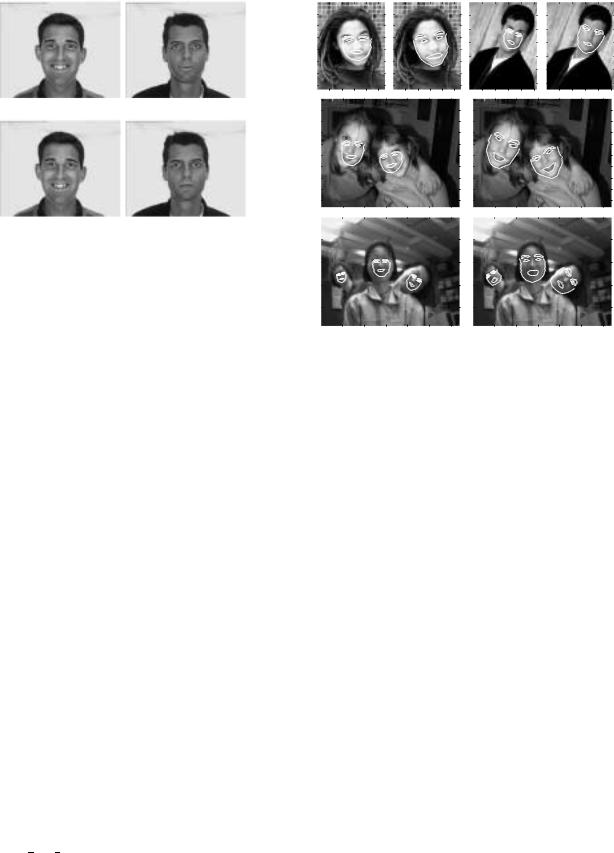
Figure 2: Comparison between BM and ASM using the same training data. (a)(b) the results of ASM; (c)(d) the results of BM.

(d)Go to step (a) unless the newly updated W is close to the old one, or the maximum iterations have been applied.

(e)if > k @, then > > @, goto (a), else exit.

Stage 2 (fine matching):

> @

(a)Calculate the internal and external energy terms, and update the contour W.

(b)Update the parameters of affine transform x (\,), the shape parameters j, and the

prototype contour WS, according to W [6]. The constraints of j is applied to ensure the prototype contour is in a plausible area.

(c)Repeat (a)(b) until convergence.

3.2Experimental Results

Face detection, extraction, and recognition plays an important role in automatic face recognition systems. In practice, the users may be expected to detect, match, or recognize faces at any angles. In this section, experiments based on facial feature extraction are presented to illustrate the effectiveness of the BM.

A contour with 89 landmark/boundary points, including six facial features: the face outline, brows, eyes, and a mouth, is recruited to describe a full face. The face images used for training are selected from the AR frontal face database [12] (http://rvl1.ecn.purdue.edu/ aleix/aleix face DB.html), which consists of various expression, male and female frontal face images. Fig.1 shows two examples of the marked faces. All the sample contours are aligned and normalized using least squares error method to constitute the shape space. The set of all the sample contours used in this experiment and

50						50						50						50
100						100
												100						100
150						150
												150						150
200						200
												200						200
250						250
												250						250
300						300
350						350						300						300
50		100	150	200	250	50		100	150	200	250		50	100	150	200	250	50		100	150	200	250

50							50
100							100
150							150
200							200
250							250
300							300
350							350
400							400
450							450
100		200	300	400	500	600	100		200	300	400	500	600
50							50
100							100
150							150
200							200
50		100	150	200	250	300	50		100	150	200	250	300

Figure 3: Examples of BM results for matching frontal faces.

the mean contour are also plotted in Fig.1. The face images used for testing are carefully selected from the database of the Vision and Autonomous System Center (VASC) of CMU (http://www.cs.cmu.edu/afs/cs.cmu.edu /user/har/Web/faces.html), representing the images with expressions, different rotation angles, and complex image background. In the experiments, the initial contours are properly placed manually as a common practice for snakes. For BM, in the coarse matching stage, facial feature points other than the outline points are passively updated according to the matching results, such that a quite large initial range of the face contour can be tolerated. Further in the fine tuning stage, all the facial feature points are utilized to give an accurate matching result of the full face. In each iteration, the contour of every facial feature is smoothed. The results of ASM is obtained by using the ASM Toolkit (Version 1.0) of the Visual Automation Ltd.

Fig. 2 shows the results obtained by using the BM and ASM models respectively, where the faces to be detected can not be seen in advance and the training data used for both the models are the same. Because ASM matches objects exactly using the reconstructed shape, it may not match the new objects accurately. For comparison, since the BM considers not only the global prior information, but also local deformations, better performance is observed from the figure. Some other experiment results, including the initial contours and the final matching results, are shown in Fig. 3. It can be seen from the figures that the BM matches the faces closely even when they are in different positions and in-plane rotation angles.

4 Conclusion

An effective deformable model, Bayesian Model, is developed in the general Bayesian framework. The global shape variation is modeled using the prior shape knowledge, and a transformational invariant internal energy is utilized to describe the shape deformations between the prototype contour and the deformable contour. Compared with the ASM algorithm, experimental results based on facial feature extraction verify the effectiveness of the proposed BM model. It also worth noting that as long as a set of training samples of object shapes is available, the BM can be applied to other applications such as object segmentation and tracking.

References

[1]A.K. Jain, Y. Zhong, and S. Lakshmanan, “Object matching using deformable templates,” IEEE Transactions on Pattern Analysis and Machine Intelligence, vol. 18, no. 3, pp. 267–278, 1996.

[2]S. Lakshmanan and D. Grimmer, “A deformable template approach to detecting straight edges in radar images,”

IEEE Transactions on Pattern Analysis and Machine Intelligence, vol. 18, no. 4, pp. 438–443, 1996.

[3]A.L. Yuille, P.W. Hallinan, and D.S. Cohen, “Feature extraction from faces using deformable templates,” International Journal of Computer Vision, vol. 8, no. 2,

pp.99–111, 1992.

[4]L.H. Staib and J.S. Duncan, “Boundary finding with parametrically deformable models,” IEEE Transactions on Pattern Analysis and Machine Intelligence, vol. 14, no. 11, pp. 1061–1075, 1992.

[5]K.F. Lai and R.T. Chin, “Deformable contours: modeling and extraction,” IEEE Transactions on Pattern Analysis and Machine Intelligence, vol. 17, no. 11, pp. 1084–1090, 1995.

[6]T.F. Cootes, C.J. Taylor, D.H. Cooper, and J. Graham, “Active shape models - their training and application,”

Computer Vision and Image Understanding, vol. 61, no. 1, pp. 38–59, 1995.

[7]T. Cootes, G.J. Edwards, and C.J. Taylor, “Active appearance models,” in Proceeding of 5th European Conference on Computer Vision, 1998, vol. 2, pp. 484–498.

[8]T.F. Cootes and C.J. Taylor, “Combining elastic and statistical models of appearance variation,” in Sixth European Conference on Computer Vision, ECCV’00, 2000,

p.149 163.

[9]B. Moghaddam and A. Pentland, “Probabilistic visual learninig for object representation,” IEEE Transactions on Pattern Analysis and Machine Intelligence, vol. 19, no. 7, pp. 696–710, 1997.

[10]S. Umeyama, “Least-squares estimation of transformation parameters between two point patterns,” IEEE Transactions on Pattern Analysis and Machine Intelligence, vol. 13, no. 4, pp. 376–380, 1991.

[11]M. Werman and D. Weinshall, “Similarity and affine invariant distances between 2d point sets,” IEEE Transactions on Pattern Analysis and Machine Intelligence, vol. 17, no. 8, pp. 810–814, 1995.

[12]A. Martinez and R. Benavente, “The AR face database,”

CVC Technical Report #24, June, 1998.