Vanguard_watermark

vk.com/id446425943

Two factors that we have built into our base case for 2019 are escalating U.S.-China trade tensions and some further moderation in China’s economic growth. Those two (interrelated) factors are already acting as a small impediment to global growth in our base case, but the risk is that they could further

undermine global demand and ultimately global growth.

We also think there is a nontrivial risk of disruption to economic activity from a flare-up of the standoff

in Europe between Italy’s government and European policymakers that, in extremis, could lead to Italy’s exit from the euro area. Brexit-related risks continue to drag on the United Kingdom’s economy and, to a lesser extent, Europe’s, but we do not see this as one of the major risks likely to lead to a global downturn.

FIGURE I-5 (continued)

Global risks to the outlook

			Vanguard assessment of risks
2019
global risks	Description	Negative scenario	Base case	Positive scenario

Euro breakup risk

An escalation in tensions relating to Italy. The risk is that the European Commission will assess penalties on Italy, which further stokes Italian resentment toward

the European Union and provokes an Italian exit from the euro.

16%

The Italian government maintains a loose fiscal policy that results in EU sanctions, prompting a political crisis and eventual departure from the euro. This results in a wider crisis in the euro area and the departure of more countries.

68%

The Italian government revises fiscal policy to abide by EU rules and market tensions subside, but public and private sector deleveraging is still minimal. Euro breakup concerns are diminished but have not disappeared.

16%

The Italian government backs down completely and submits a fiscal austerity plan that causes public debt to fall more quickly than currently expected and euro breakup concerns to subside.

Emergingmarket debt crises

Key drivers of emerging-market cycles are global monetary divergence, the effect of the U.S. dollar on dollardenominated debt, and global/China demand for commodities.

24%

Trade wars, a slowdown of the Chinese economy, or a strong U.S. dollar due to continued divergence of monetary policy lead to spillovers and broader emerging-market crises.

57%	19%
Emerging-market debt	U.S. dollar level
crises remain contained	normalizes as
to a few idiosyncratic	developed-market
cases. Global monetary	central banks
convergence and the	commence
stabilization of the	normalization. Risk-on
Chinese economy ease	environment helps
the risk of contagion to	emerging markets
all emerging markets.	undergo V-shape
	bounce-back.

Note: Odds for each scenario are based on median responses to a poll of Vanguard’s Global Economics and Capital Markets Outlook Team. Source: Vanguard.

11

vk.com/id446425943

Global growth outlook: Moderating to trend

Vanguard dashboards of leading economic indicators and implied economic growth for 2019

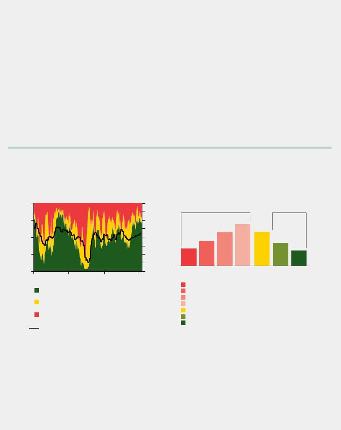
United States: Above trend but falling

Our proprietary U.S. leading indicators dashboard

is a statistical model based on more than 80 leading economic indicators from major sectors of the U.S. economy. As Figure I-6a shows, in spite of a high proportion of green indicators (above-trend readings) in the dashboard at present, there is an incipient increasein red indicators, signaling the start of a gradual slowdown in the U.S. economy. The most positive (green) indicators are those associated with increased

business and consumer confidence, a tightening labor market, and a stronger manufacturing sector. The negative (red) indicators are associated with trade balance, disposable personal income, and mortgage applications. Building permits and new-vehicle sales are below trend but show positive momentum (yellow indicators).

Using regression analysis, we mapped our proprietary indicators to a distribution of potential scenarios for U.S. economic growth in 2019, as shown in Figure I-6b. The odds of growth at or exceeding 3% in 2019 (38%) are lower than the odds of growth slowing down (62%). Our base case is for U.S. growth to moderate toward its long-term trend of 2%.

Figure I-6

a. Economic indicators

b. Estimated distribution of U.S. growth outcomes

trend	100%
above/below	75
	50
Indicators	25
	0
	2000	2006	2012	2018

			Odds of a	2018	Odds of an
	10%	over-year)	slowdown	growth	acceleration
			62%	18%	20%
	8
	6			22%
	4	(year-	18%
	2		13%
		growth			12%
	0		9%		8%
	–2
		GDP
	–4
		Real
	–6

Above-trend growth: Business and consumer con dence, manufacturing surveys, industrial production

Below trend, but positive momentum: Building permits, new-vehicle sales

Below trend and negative momentum: Trade balance, disposable personal income, mortgage applications

Real GDP growth year-over-year (right axis)

Recession: Less than 0% Slowdown: 0% to 1% Moderation: 1% to 2%

Below recent trend: 2% to 3% 2018 growth: 3% to 4% Acceleration: 4% to 5% Overheating: More than 5%

Notes: Distribution of growth outcomes generated by bootstrapping the residuals from a regression based on a proprietary set of leading economic indicators and historical data, estimated from 1960 to 2018 and adjusting for the time-varying trend growth rate. Trend growth represents projected future estimated trend growth.

Source: Vanguard calculations, based on data from Moody’s Analytics Data Buffet and Thomson Reuters Datastream.

12

vk.com/id446425943

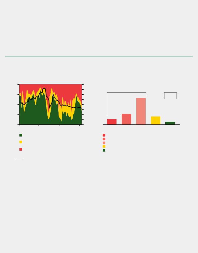
China: Continued deceleration

China is expected to continue its modest deceleration in 2019, with risks tilted to the downside, according to our proprietary China leading indicators dashboard (Figure I-6c). Specifically, despite ongoing policy efforts to stabilize near-term economic growth and combat international headwinds (as evident in improving fixed

asset investment and commodity production), yellow and

red indicators associated with softening sentiment and worsening asset returns suggest that more-aggressive stimulus measures may be needed to bolster private enterprise. Against this backdrop, China’s economy

is expected to grow by about 6%–6.3% in 2019 (Figure I-6d), with the risks of a downside slightly greater than those of a growth acceleration.

Figure I-6 (continued)

c. Economic indicators

d. Estimated distribution of China growth outcomes

trend	100%
above/below	75
	50
Indicators	25
	0
	2000	2006	2012	2018

	16%	over-year)	Odds of a	2018	Odds of an
			slowdown	growth	acceleration
	14		80%	15%	5%
	12			50%
	10	(year-
	8
		growth
	6		20%
	4			15%
		GDP	10%
	2				5%
		Real
	0

Above-trend growth:

Freight traf c, construction, loan demand

Below trend, but positive momentum:

Fixed income yields, steel production

Below trend and negative momentum:

Business climate index, future income con dence, automobile sales

Real GDP growth year-over-year (right axis)

Hard landing: Less than 5% Slowdown: 5% to 6% Deceleration: 6% to 6.5% 2018 growth: 6.5% to 7% Overheating: More than 7%

Notes: Distribution of growth outcomes generated by bootstrapping the residuals from a regression based on a proprietary set of leading economic indicators and historical data, estimated from 1960 to 2018 and adjusting for the time-varying trend growth rate. Trend growth represents projected future estimated trend growth.

Source: Vanguard calculations, based on data from CEIC and Thomson Reuters Datastream.

13

vk.com/id446425943

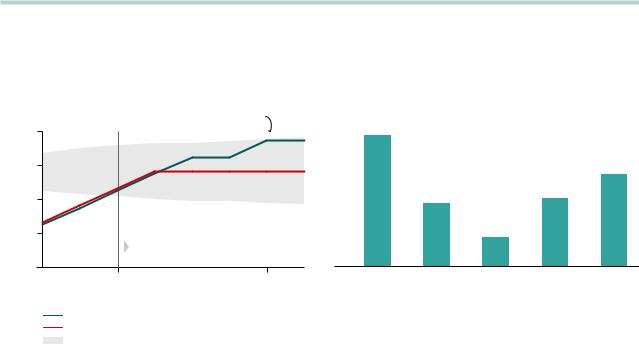
Euro area: Above trend but falling

The euro area is expected to grow at a moderate rate of about 1.5% in 2019, which is slightly above trend. As

illustrated by our leading indicators dashboard (Figure I-6e), the proportion of indicators that are tracking above trend fell throughout 2018, primarily driven by a weaker industrial sector and net trade. A slowdown in the global trade and industrial cycle, in addition to delays in German car production, explains most of this deterioration in economic momentum; German exports and German industrial

production are both currently in the red category, indicating below-trend growth and negative momentum. We expect growth to stabilize in the first half of 2019 as car production recovers. Moreover, a large proportion of leading indicators are still in green territory, including business

and consumer sentiment, labor market data, and monetary policy. This should provide support to growth next year. However, as shown in Figure I-6f, the risks to the growth outlook are skewed to the downside given China’s continuing slowdown, U.S.-China trade tensions, and elevated political risks concerning Brexit and Italy.

Figure I-6 (continued)

e. Economic indicators

f. Estimated distribution of euro-area growth outcomes

trend	100%
above/below	75
	50
Indicators	25
	0
	2000	2006	2012	2018

	8%	over-year)	Odds of a	2018	Odds of an
			slowdown	growth	acceleration
	6		35%	45%	20%
	4
		(year-
	2
	0	growth	25%
	–2				15%
		GDP	10%
	–4
					5%
		Real
	–6

Above-trend growth: Business and consumer con dence, interest rates, employment growth

Below trend, but positive momentum:

Building permits, real wages

Below trend and negative momentum:

Industrial production, export growth, new factory orders

Real GDP growth year-over-year (right axis)

Recession: Less than 0% Slowdown: 0% to 1% 2018 growth: 1% to 2% Acceleration: 2% to 3%

Overheating: More than 3%

Notes: Distribution of growth outcomes generated by bootstrapping the residuals from a regression based on a proprietary set of leading economic indicators and historical data, estimated from 1960 to 2018 and adjusting for the time-varying trend growth rate. Trend growth represents projected future estimated trend growth.

Source: Vanguard calculations, based on data from Bloomberg and Macrobond.

14

vk.com/id446425943

United States: Going for a soft landing

Much of our global outlook hinges on our expectations for conditions in the United States. In 2019, U.S. economic growth should decline from current levels toward trend growth of about 2%. While we believe a recession remains some time off (see Figure I-2

on page 7), we expect the U.S. labor market will cool, with employment growth falling closer in line with the trend growth of the labor force (80,000–100,000 per month), and structural factors such as technology and globalization should prevent inflation from rising significantly above the Federal Reserve’s 2% target.

The strong performance of the U.S. economy over the last two years is in part explained by significant support from expansionary monetary and fiscal policies. We estimate that the latter contributed over 50 basis points to headline growth in 2018. (A basis point is one-hundredth of a percentage point.) In 2019, we expect monetary policy to dial back to “neutral,” with the federal funds rate reaching 2.75%–3% in June of

2019. On the fiscal policy front, we may continue to see the expansionary effects of the Tax Cuts and Jobs Act through the first part of the year. However, we expect the boost to the year-over-year GDP growth rates from consumer spending to begin fading away toward the second half.

But the strong performance of the U.S. economy has been due to more than just policy. The U.S. consumer has been the key engine of growth during the recovery from the global financial crisis, with almost all drivers of spending firing on all cylinders, including recent support from lower income-tax payroll withholdings (see Figure I-7). Looking ahead to 2019, the dashboard gets a bit more muddled. Nothing is flashing red, but,

with the exception of household debt measures and wage growth, all indicators get worse. Higher interest rates will start to bleed through to mortgage rates and rates for auto and personal loans. They will also affect asset valuations in credit-sensitive sectors such as housing.

On the jobs front, it will be hard for the U.S. economy

FIGURE I-7

Dashboard of consumer drivers

	2017/
	2018	2019 Assessment
	Wage growth	Further improvement in wages will be limited by low labor productivity growth
	Jobs (growth, lower	Employment growth will level off
	unemployment)
	Household debt to disposable	Outstanding debt and the cost of servicing it will remain low
	income

High equity valuations and market volatility on the rise could be a drag Wealth effects on financial wealth. Rising rates will affect credit-sensitive sectors, including

home prices. Year-over-year tax cuts will disappear.

	Interest rates and cost of credit	Mortgage rates and rates for auto and personal loans will rise
	Consumer confidence	Unknown; policy uncertainty and market volatility will rise
	Consumer prices	Inflation will stay close to the Fed’s target
	(inflation and import prices)
	Source: Vanguard’s Global Economics and Capital Markets Outlook Team.

15

vk.com/id446425943

to replicate the impressive pace of job creation of the last two years. While the labor market will stay strong, it may not provide similar contributions to growth

in 2019. And several unknowns such as trade policy uncertainty, increased market volatility, and high equity valuations will possibly affect consumer confidence and stock market wealth.

One of the most puzzling aspects of an otherwise strong U.S. economy continues to be subpar wage growth. As the unemployment rate (3.7% as of November 2018) has fallen to the lowest level since the 1960s, why does wage growth, which is only now reaching 3%, remain so tepid by historical standards?

All else equal, stronger demand for workers should result in higher wages, but all else is not equal. Fundamentally, we should not expect inflation-adjusted (real) wages to exceed the levels of labor productivity

growth and inflation. Productivity growth rates have been (1% since the recovery began in 2010, compared with 2% before the global financial crisis. This means we should not expect pre-crisis levels of wage growth, particularly after incorporating inflation, which has struggled to consistently achieve the Fed’s 2% target (see Figure I-8).1

While low labor productivity can explain subdued real wage growth, one concern that investors have for 2019 is that ever tighter labor markets could eventually fuel a wage-inflation spiral involving nominal wages and final consumer prices. The concern is rooted in the strong historical relationship between nominal wages and inflation. However, as shown in Figure I-9a, the beta

of nominal wage growth on consumer inflation has declined significantly since the 1990s. At the core of this shift in the wage-inflation relationship is the Fed’s ability to manage inflation expectations effectively. If they

FIGURE I-8

Absent a significant increase in productivity, higher wage growth is unlikely

	3.5%
year)	3.0
	2.5
over-
(year-	2.0
rates	1.5
Growth	1.0
	0.5
	0
	1990	1992	1994	1996	1998	2000	2002	2004	2006	2008	2010	2012	2014	2016	2018

Real wage growth (trend)

Real wage growth

Labor productivity growth (trend)

Notes: Real wage growth is calculated as the growth rate of hourly wages as reported in the Employment Cost Index (ECI) minus core PCE inflation rate for that year. Trend for real wage growth is estimated as a centered three-year moving average of real wage growth.

Sources: Congressional Budget Office, Bureau of Labor Statistics.

16 1 See the 2017 Vanguard Global Macro Matters paper Why Is Inflation So Low? The Growing Deflationary Effects of Moore’s Law.

vk.com/id446425943

remain in check, workers would have little reason to fear high inflation and thus would not demand higher nominal wages above and beyond any labor productivity gains plus reasonable levels of inflation around the Fed’s 2% target. If wage gains keep pace with productivity and inflation expectations remain near the Fed’s target, unit labor costs for businesses would not rise faster than inflation and there would be no impact on final consumer prices.

Inflation expectations and the Fed’s ability to manage them (that is, the Fed’s credibility) are often overlooked in Phillips curve models that correlate rising inflation with low unemployment. Figure I-9b shows our inflation estimates from an augmented Phillips curve model that incorporates not only labor market slack but also inflation expectations and other secular forces affecting inflation, such as globalization and technology.2 Core inflation is projected to hover closely near the Fed’s inflation target in 2019.

Yet it is this Phillips curve logic that has many who are attempting to anticipate the Fed’s next move very focused on the labor market. However, in 2019, the Fed will be able to worry less about the unemploymentinflation link by leaning heavily on its credibility with the market. It will instead rely more on its assessment of a neutral policy stance as its guiding principle.

Calibrating policy rates to neutral is an extremely complex exercise full of risks. The so-called soft landing requires significant skill by policymakers. The neutral rate (usually referred to as r*) is a moving target and not directly observable, as it has to be estimated with statistical models. The Fed’s extremely gradualist approach during this rate-hiking cycle does help increase the odds of a successful landing this time, however. Our best attempt to estimate the neutral rate places it somewhere in the 2.5%–3% range. If this is correct, the Fed is likely to

FIGURE I-9

Runaway inflation remains unlikely

a. Pass-through of earnings to inflation has waned	b. An “augmented” Phillips curve model
with anchored inflation expectations

		1.4
		1.2
ationin growth		1.0
		0.8
		0.6
Sensitivity of	to earnings
		0.4
		0.2
		0
		–0.2
		–0.4
		1970	1978	1986	1994	2002	2010	2018

Notes: Figure indicates the sensitivity of core PCE inflation to year-over-year growth in average hourly earnings using rolling ten-year regression coefficients. Data cover January 1960–September 2018.

Sources: Vanguard calculations, Moody’s Analytics Data Buffet.

Forecast

In ation will

in ationin	3.0%	Fed’s	struggle to
			achieve the Fed’s
	2.5	target	target in 2019
	2.0
year change
	1.5
	1.0
over-	0.5
Year-	0
	2000	2006	2012	2018

Year-over-year core PCE

Model forecast

Notes: Core PCE model is a root mean square error (RMSE)-weighted average of two models: a bottom-up model where we model the deviation of augmented Phillips curve fitted values to each major component in the core PCE and a topdown macro model. The RMSE is 0.35 for the bottom-up model and 0.24 for the top-down model. This leads to a 40% weight for the bottom-up model and a 60% weight for the top-down model in the weighted model.

Source: Vanguard calculations, based on Thomson Reuters Datastream, Bureau

of Economic Analysis, Bureau of Labor Statistics, Philadelphia Federal Reserve Bank Survey of Professional Forecasters, Congressional Budget Office, and Bloomberg Commodity Index.

2 See the 2018 Vanguard Global Macro Matters paper From Reflation to Inflation: What’s the Tipping Point for Portfolios?

17

vk.com/id446425943

increase the policy rate to a range of 2.75%–3% by June of 2019 and then stop or at least pause to reassess conditions.

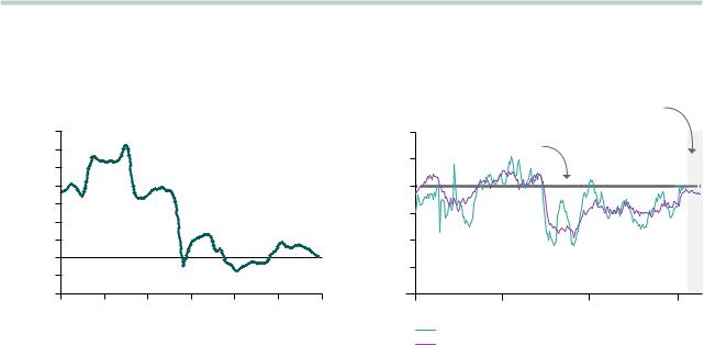
The risks to our view are not negligible. Historically, the U.S. Treasury yield curve has provided one of the clearest real-time indicators of overly tight policy. If policy becomes too restrictive, the slope of the yield curve falls, and at some point before a recession, it inverts.3 Inversion typically occurs when the market believes the Fed has gone too far and drives the yield

of the 10-year Treasury below the federal funds rate and

that of the 3-month Treasury yield. Recession typically ensues 12 to 18 months later. Since the onset of policy rate increases in 2015, the slope of the Treasury curve has flattened from 300 basis points to around 80 basis points today. As the Fed continues to normalize policy in 2019, the risks of inversion will build (Figure I-10a).

Some subscribe to the view that a new policy environment means that a flatter yield curve does not hold the same predictive power it once did. Our research leads us to believe that while this power has diminished over time, it still presents a fairly significant risk to our 2019 U.S. base case.4

FIGURE I-10

The yield curve remains a relevant leading indicator of economic growth

a. Further flattening expected; inversion risk increases in 2019

b. Relationship of growth to yield curve has not deteriorated in the quantitative-easing era

		Increased
	3.5%	policy risk
rate	3.0
Interest	2.5
	2.0	Elevated inversion
	1.5	risk past this point
	Q1	Q1
	2019	2020

Fed FFR expectations

ISG FFR expectations

VCMM projected U.S. 10-year Treasury path

Notes: FFR refers to federal funds rate. The U.S.10-year Treasury path range uses the 35th to 65th percentile of projected VCMM path observations. Distribution of return outcomes is derived from 10,000 simulations for each modeled asset class. Simulations are as of June 30, 2018. Results from the model may vary with each use and over time.

Sources: Vanguard calculations, based on data from Thomson Reuters Datastream and Moody’s Analytics Data Buffet; Federal Reserve Bank of New York.

0.27
cientcoef				0.19
	0.13		0.14
Regression
		0.06
1970s	1980s	1990s	2000 to	2008 to
			2007	2018

Sensitivity of growth to yield curve

Notes: Data are through June 30, 2018. Sensitivity is represented by coefficients from an ordinary least squares (OLS) regression model of yield curve slope (10-year U.S. Treasury yield minus 3-month T-bill yield) and the Vanguard Leading Economic Indicators series (used as a proxy for growth with monthly observations) 12 months forward. Coefficients are statistically significant at the 1 percent significance level.

Source: Vanguard calculations, based on data from Moody’s Analytics Data Buffet and Thomson Reuters Datastream.

3 As measured by the difference between 3-month and 10-year constant-maturity Treasury yields.

18 4 See the 2018 Vanguard Global Macro Matters paper Rising Rates, Flatter Curve: This Time Isn’t Different, It Just May Take Longer.

vk.com/id446425943

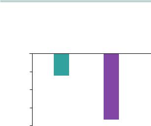
Outside of monetary policy, the largest domestic risk to our U.S. outlook stems from trade policy. Trade represents a relatively small proportion of the U.S. economy (20% of GDP vs. a developed-market average of 35%). However, if trade tensions reverberate through financial markets (as shown in increases in the BBB spread in Figure I-11), the implications for economic conditions, including growth, become more significant. While we believe the U.S. will avoid recession in 2019, if the impacts of monetary and trade policies spread to financial markets, the likelihood of a downturn will become more substantial.

FIGURE I-11

Trade war impacts

GDP impact of higher costs of traded goods and financial market uncertainty

		0
Impact on annualized	quarterly GDP growth	–0.1
			Baseline
		–0.2
		–0.3
		–0.4	Future
			escalation

Baseline: A 25% tariff on $350 billion in imported goods (approximate amount of the U.S. trade deficit with China) and a retaliatory 25% tariff on $350 billion in exported goods along with a 25-basis-point widening of the credit spread.

Further escalation: A 25% tariff on a further $200 billion in imported goods (approximate amount of automobile, steel, and aluminum imports exposed to announced tariffs) and retaliatory 25% tariff on a further $200 billion in exported goods along with a 100-basis-point widening of the credit spread.

Notes: Tariff impacts are based on increasing prices of imports and exports by percentage indicated in the Federal Reserve’s FRB/US model. The credit spread is the BBB spread. BBB spread impacts are based on shocking the yield

spread of long-term BBB corporate bonds versus the 10-year Treasury bond yield by the indicated percentage.

Source: Vanguard calculations, based on the Federal Reserve’s FRB/US Model.

Euro area: Stable growth as policy normalizes

After a sharp slowdown in 2018, euro-area growth is likely to stabilize around 1.5% in 2019, which is slightly above trend (see Figure I-6f on page 14). The slowdown was exacerbated by weak global demand for euro-area exports and delays to German car production as carmakers adjust to new European Union (EU) emissions standards.

In early 2019, we expect growth to modestly rebound as car production gets back on track. In addition, domestic demand in the euro area is likely to remain resilient, supported by healthy levels of business and consumer confidence and very low interest rates, which should continue to stimulate demand for credit. A stronger rebound remains unlikely in our view, given

China’s ongoing slowdown and U.S.-China trade tensions, which will weigh on demand for euro-area exports.

In 2019, risks to the euro area are tilted slightly to the downside, given a number of important global risks we outlined in the global growth outlook section. Domestically, the biggest risk is a further escalation in tensions between Italy’s government and European policymakers. In 2019, Italy may break the 3% fiscaldeficit ceiling imposed on all EU members, and given the recent downgrade of Italian sovereign debt by key

ratings agencies and the associated rise in Italian bond yields, Italy’s debt levels are likely to remain elevated for the foreseeable future. Nervousness about Italy’s fiscal position may spill over to other Italian assets and to periphery bond markets, which on its own could dampen growth. The larger risk, however, is that the European Commission imposes penalties on Italy, further stoking Italian resentment toward the EU and provoking Italy

to exit from the euro. We think the chance of an Italian exit is only 5% over the next five years, but the situation warrants close attention.

19

vk.com/id446425943

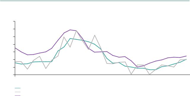
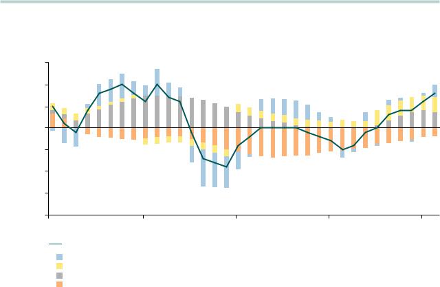
In 2019, we expect the labor market to continue tightening, given that growth is likely to remain above trend for most of the year. The unemployment rate, now close to 8%, is likely to approach 7.5% by year-end, leading to a further lift in wage growth and core inflation (Figure I-12a).

At this stage, we see a low probability of a surprise surge in core inflation, for two key reasons. First, Germany’s economy is becoming deeply integrated with low-wage countries in Central and Eastern Europe, so German firms will be unwilling to offer higher wages at home. Second, periphery countries such as Italy, Spain, and Portugal need to contain their labor costs to restore competitiveness with the more efficient German economy.

Given this environment of tightening labor markets and rising inflation pressures, we expect the European Central Bank (ECB) to lift interest rates for the first time in late 2019 (Figure I-12b). By that stage, we estimate that the output gap will be slightly positive, with core

inflation on track to reach target over the short to medium term. This will be followed by a very gradual hiking path thereafter (25 basis points every six months), given that we do not anticipate strong price pressures, as outlined above. Our analysis suggests that core inflation is unlikely to reach the ECB’s target until wage growth increases.

FIGURE 1-12

European wage pressures are building, which will prompt the ECB to initiate a gradual hiking cycle

a. Drivers of euro-area wage growth

		1.5
Percentage point contributions to	deviation from mean wage growth	1.0
		0.5
		0
		–0.5
		–1.0
		–1.5
		–2.0
		2010	2012	2014	2016	2018

Compensation per employee

Unexplained

Productivity

Past in ation

Labor market slack (unemployment rate-NAIRU)

Notes: This decomposition has been derived from an OLS regression of compensation per employee on productivity growth, past inflation, and labor market slack. The nonaccelerating inflation rate of unemployment (NAIRU) is derived from the estimate by the Organisation for Economic Co-operation and Development (OECD).

Source: Vanguard calculations, based on data from Eurostat and the OECD.

20