Название-Сеть в Играх 2006год_Язык-Eng

64 Networking and Online Games: Understanding and Engineering Multiplayer Internet Games

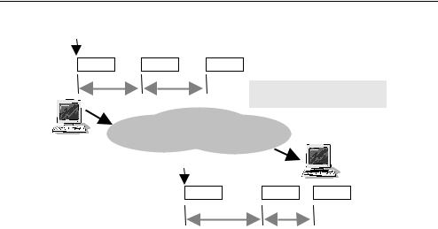
manually configured to map 128.80.6.200:28000 to 192.168.0.13:27960. The master server ‘sees’ the Quake III Arena server at 128.80.6.200:28000. However, without special configuration the NAT/NAPT router will not allow new players to actually connect through 128.80.6.200:28000 to the game server itself. We discuss this again in Chapter 12.)

NAT/NAPT has its admirers and detractors. Nevertheless, it does serve a purpose for private networks that cannot afford lots of public IP addresses or wish to avoid renumbering of their internal networks on a regular basis.

Consumer home routers/gateways invariably support some form of NAT/NAPT functionality. Demand is driven by the deployment of broadband IP access over Asymmetric Digital Subscriber Line (ADSL) or cable modem services, and the fact that many homes have multiple computers. Typically the home router has one Ethernet port to the ADSL modem or cable modem, and one or more Ethernet ports for the internal, home network. (To assist in address management of a small home network, many home routers also support the dynamic host configuration protocol described in the following section.)

4.3.3 Dynamic Host Configuration Protocol

The DHCP [RFC2131] automates the configuration of various fundamental parameters hosts need to know before they can become functional members of an IP network. For example, every host minimally needs to know the following:

•The host’s own IP address

•The subnet mask for the subnet on which it sits

•The IP address of at least one router to be used as the default route for all traffic destined outside the local subnet.

Without these pieces of information, a host cannot properly set the source IP address of its outbound packets, cannot know if it is the destination of inbound unicast packets, and cannot build a basic forwarding table that differentiates between on-link and off-link next hops.

DHCP allows hosts to automatically establish the preceding information, and provides two key benefits:

•The need for manual intervention is minimised when installing and turning on new hosts.

•IP addresses can be leased for configurable periods of time to temporary hosts.

Minimising administrative burdens clearly saves money and time, and increases overall convenience. The benefits of dynamic address leasing become apparent in networks where not all hosts are attached and operational at the same time.

4.3.3.1 Configuring a Host

DHCP is a client–server protocol. Each host has a DHCP client embedded in it, and the local network has one or more nodes running DHCP servers. DHCP runs on top of UDP, which at first glance suggests a Catch-22 situation with the unconfigured IP

Basic Internet Architecture	65

interface. However, DHCP only requires that an unconfigured IP interface can transmit a broadcast packet (IP destination address ‘255.255.255.255’) to all other IP interfaces on the local link.

A DHCP client solicits configuration information through a multistep process:

•First the client broadcasts a DHCP Discover message in a UDP packet to port 67, to identify its own link layer address and to elicit responses from any DHCP servers on the local network.

•One or more DHCP servers reply with DHCP Offer messages, containing an IP address, subnet mask, default router, and other optional information that the client may use to configure itself [RFC2132].

•The DHCP client then selects one of the servers, and negotiates confirmation of the configuration by sending back a DHCP Request to the selected server.

•The selected DHCP server replies with a DHCP Ack message, and the host begins operating as a functional member of the subnet to which it has been assigned.

Address administration is thus centralised to one or more DHCP servers.

4.3.3.2 Leasing Addresses

DHCP servers may be configured to allocate IP addresses in a number of ways:

•Static IP mappings based on a priori knowledge of the link layer addresses of hosts supposed to be on the managed subnet.

•Permanent mappings that are generated on-demand (the server learns client link layer addresses as clients announce themselves).

•Short-term leases, where the DHCP client is assigned an IP address for a fixed period of time after which the lease must be renewed or the address returned to the server’s available address pool.

The third option is most useful where network access must be provided to a large group of transient hosts using a smaller pool of IP addresses. For example, consider a public access terminal centre at a university with 50 Ethernet ports into which students can plug their laptop computers. Many hundreds or thousands of students might use the centre over a week or a month. Thousands of IP addresses would be required for a static IP address assignment scheme, one for each student’s laptop. On the contrary, leasing addresses for short periods of time means that a much smaller pool of IP addresses can serve the terminal centre’s needs.

A DHCP server can specify lease times in the order of hours, days, or weeks with a minimum lease time of one hour. DHCP clients are informed of the lease time when they first receive their address assignment. As the lease nears expiration, DHCP clients are expected to repeat the Request/Ack sequence to renew their lease. The DHCP server usually allows clients to continue with their leases at renewal.

DHCP clients are also allowed to store their assigned IP address in long-term storage (battery-backed memory, or local disk drive) and request the same address again when it next starts up. If the address has not subsequently been issued to another client, DHCP servers typically allow a lease to be renewed after clients go through a complete restart.

66 Networking and Online Games: Understanding and Engineering Multiplayer Internet Games

4.3.4 Domain Name System

As noted earlier in this chapter, IP addresses are not the same as FQDNs (often referred to simply as domain names). Domain names are human-readable, text-form names that indirectly represent IP addresses.

The DNS is a distributed, automated, hierarchical look-up and address mapping service [RFC1591]. People typically use domain names to inform an application of a remote Internet destination, and the applications then use the DNS to perform on-demand mappings of domain names to IP addresses. This level of indirection allows consistent use of well-known domain names to identify hosts, while allowing a host’s IP address to change over time (for whatever reason).

Two forms of hierarchy exist in the DNS – hierarchy in the structure of names themselves and a matching hierarchy in the distributed look-up mechanism.

4.3.4.1 Domain Name Hierarchy

Domain names are minimally of the form name . tld where tld specifies one of a handful of Top Level Domains (TLDs) and name is an identifier registered under the specified top-level domain. Examples of generic three letter TLDs (gTLDs) include com, edu, net, org, int, gov, and mil. Country code TLDs (ccTLDs) are constructed from standard ISO-3166 two letter ‘country codes’ (e.g. au, uk, fr, and so on) [ISO3166].

The nested hierarchy is read from right to left, and name may itself be broken up into multiple levels of subdomains. Some TLDs are relatively flat (for example, the ‘com’ TLD), with companies and originations around the world able to register second-level domains immediately under ‘com’. Country code TLDs have varied underlying structures, sometimes replicating a few of the existing three letter TLDs as second-level domains (for example, Australia registers domain names under a range of second-level domains including ‘com.au’, ‘edu.au’, and so on.)

The hierarchical structure reflects the administrative hierarchy of authority associated with assigning names to IP addresses. For example, consider an address like ‘mail.accounting.bigcorp.com’. The managers for ‘com’ have delegated all naming under ‘bigcorp.com’ to a second party (most likely the owners of ‘BigCorp, Inc.’). BigCorp no doubt has various internal departments, including the Accounting department. Someone in the accounting department has been delegated authority for naming under ‘accounting.bigcorp.com’, and they have assigned a name for the mail server in the accounting department. Figure 4.18 represents the relationships between the subdomains discussed so far.

A domain name hierarchy is independent of the hierarchy of IP addresses and subnets discussed earlier in this chapter. For example, onemachine.bigcorp.com might well be on an entirely different IP subnet (indeed, even a different country) from othermachine.bigcorp.com.

Domain name registration has become a commercial business in its own right, and multiple registrars jointly manage different sections of the DNS. Up-to-date information on registrars and domain assignment policies can be found in the Internet Assigned Numbers Authority web site, http://www.iana.org.

Basic Internet Architecture					67
Top-level	.com	.edu	.org	.au
domains
.bigcorp.com			.iana.org	.com.au	.edu.au
.accounting

.bigcorp.com	www.iana.org

mail.accounting

.bigcorp.com

Figure 4.18 Hierarchy within domain name structure reflects a hierarchy of delegation authority

4.3.4.2 DNS Hierarchy

The hierarchy in a domain name essentially describes a search path across the distributed collection of name servers that together make up the Internet’s DNS. Name servers are queried whenever a domain name needs to be resolved to an IP address. Certain name servers are responsible for being authoritative sources of information for particular domains or subdomains. The name servers ultimately responsible for each TLD are known as root name servers.

Before hosts can use the DNS they must be configured with the IP address of a local name server – the host’s entry point into the DNS. The ISP or whoever supports your network typically provides the local name server. The name server’s IP address is either manually configured into each host, or can be automatically configured (for example, DHCP provides an option for configuring the local name server’s address [RFC2132]).

Local name servers are manually configured to know the IP address of at least one root name server, and possibly another name server further up the domain name tree. Name servers either answer queries with local knowledge, or seek out another name server who is responsible for mappings higher up the domain name hierarchy. Local knowledge is often held in a cache built from recent queries from other hosts – the cache allows rapid answers for frequently resolved domain names.

For the curious reader: Many recent versions of Windows, and Unix-link operating systems such as Linux and FreeBSD have a tool called nslookup. Often installed as a command line application, nslookup allows you to manually perform DNS queries and explore your local network’s DNS configuration. Similar tools may be found under names like dig or host.

References

[ISO3166] http://www.iso.org/iso/en/prods-services/iso3166ma/02iso-3166-code-lists/list-en1-semic.txt. [RFC768] J. Postel, Ed, “User Datagram Protocol”, RFC 768. August 1980.

[RFC791] J. Postel, Ed, “Internet Protocol Darpa Internet Program Protocol Specification”, RFC 791. September 1981.

68 Networking and Online Games: Understanding and Engineering Multiplayer Internet Games

[RFC793] J. Postel, Ed, “Transmission Control Protocol”, RFC 793. September 1981.

[RFC826] D.C. Plummer, “An Ethernet Address Resolution Protocol”, RFC 826. November 1982. [RFC1112] S. Deering, “Host Extensions for IP Multicasting”, RFC 1112. August 1989. [RFC1191] J. Mogul, S. Deering, “Path MTU Discovery”, RFC 1191. November 1990.

[RFC1390] D. Katz, “Transmission of IP and ARP over FDDI Networks”, RFC 1390. January 1993. [RFC1519] V. Fuller, T. Li, J. Yu, K. Varadhan, “Classless Inter-Domain Routing (CIDR): an Address Assign-

ment and Aggregation Strategy”, RFC 1519. September 1993.

[RFC1591] J. Postel, “Domain Name System Structure and Delegation”, RFC 1591. March 1994. [RFC1771] Y. Rekhter, T. Li, “A Border Gateway Protocol 4 (BGP-4)”, RFC 1771. March 1995.

[RFC1918] Y. Rekhter, B. Moskowitz, D. Karrenberg, J. de Groot, E. Lear, “Address Allocation for Private Internets”, RFC 1918. February 1996.

[RFC1981] J. McCann, S. Deering, J. Mogul, “Path MTU Discovery for IP version 6”, RFC 1981. August 1996.

[RFC2003] C. Perkins, “IP Encapsulation within IP”, RFC 2003. October 1996. [RFC2004] C. Perkins, “Minimal Encapsulation within IP”, RFC 2004. October 1996.

[RFC2050] K. Hubbard, M. Kosters, D. Conrad, D. Karrenberg, J. Postel, “Internet Registry IP Allocation Guidelines”, RFC 2050. November 1996.

[RFC2131] R. Droms, “Dynamic Host Configuration Protocol”, RFC 2131. March 1997.

[RFC2132] S. Alexander, R. Droms, “DHCP Options and BOOTP Vendor Extensions”, RFC 2132. March 1997.

[RFC2225] M. Laubach and J. Halpern, “Classical IP and ARP over ATM”, Internet Request for Comment 2225. April 1998.

[RFC2328] J. Moy, “OSPF Version 2”, RFC 2328. April 1998. [RFC2453] G. Malkin, “RIP Version 2”, RFC 2453. November 1998.

[RFC2473] A. Conta, S. Deering, “Generic Packet Tunneling in IPv6 Specification”, RFC 2473, December 1998.

[RFC2616] R. Fielding, J. Gettys, J. Mogul, H. Frystyk, L. Masinter, P. Leach, T. Berners-Lee, “Hypertext Transfer Protocol – HTTP/1.1”, RFC 2616. June 1999.

[RFC2821] J. Klensin, Ed, “Simple Mail Transfer Protocol”, RFC 2821. April 2001. [RFC2993] T. Hain, “Architectural Implications of NAT”, RFC 2993. November 2000.

[RFC3022] P. Srisuresh, K. Egevang, “Traditional IP Network Address Translator (Traditional NAT)”, RFC 3022. January 2001.

[IANAP] Internet Assigned Numbers Authority, “Directory of General Assigned Numbers (last viewed January 2006)”, http://www.iana.org/numbers.html.

[8023] IEEE Std 802.3. “IEEE Standards for Local and Metropolitan Area Networks: Specific Requirements. Part 3: Carrier Sense Multiple Access with Collision Detection (CSMA/CD) Access Method and Physical Layer Specifications”, 1998.

5

Network Latency, Jitter and Loss

Regardless of game genre, the realism of online game play depends on how well the underlying network allows game participants to communicate in a timely and predictable manner. In the previous chapter, we broadly reviewed the nature of modern IP network services. In this chapter we will discuss in more detail three characteristics of best effort Internet Protocol (IP) service – latency, jitter and loss – that have a significant impact on game play experience and game design. We will also look briefly at the technical methods Internet Service Providers (ISPs) can utilise to control these characteristics of their network services.

5.1 The Relevance of Latency, Jitter and Loss

As noted in the previous chapter, IP packets carry information between sources and destinations on the network. Latency refers to the time it takes for a packet of data to be transported from its source to its destination. In many networking texts, you will also see the term Round Trip Time (RTT) in reference to the latency of a round trip from source to destination and then back to source again. In many cases the RTT is twice the latency, although this is not universally true (some network paths exhibit asymmetric latencies, with higher latencies in one direction than the other). In online gaming communities, the term lag is often colloquially used to mean RTT.

Variation in latency from one packet to the next is referred to as jitter. There are a number of mathematically precise ways to define jitter, usually depending on the timescale over which the latency variation occurs and the direction in which it occurs. For example, a path showing an average 100 ms latency might exhibit latencies of 90 ms and 110 ms for every alternate packet – fairly noticeable jitter in the short term, even though the long-term average latency is constant. Alternatively, the path might exhibit latency, that is, drifting – 90 ms, 95 ms, 100 ms, 105 ms, 110 ms, 105 ms, 100 ms. . . and so on. For our purposes, it is sufficient to know that latency can fluctuate slowly or rapidly from one packet to the next.

Figure 5.1 summarises the key difference between latency and jitter.

Packet loss refers to (not surprisingly) the case when a packet simply never reaches its destination. It is lost somewhere in the network. A path’s packet loss characteristic is often described in terms of packet loss rate or packet loss probability (ratio of the number of packets lost per number of packets sent).

Networking and Online Games: Understanding and Engineering Multiplayer Internet Games

Grenville Armitage, Mark Claypool, Philip Branch 2006 John Wiley & Sons, Ltd

70 Networking and Online Games: Understanding and Engineering Multiplayer Internet Games

Time t1
Packet 1	Packet 2	Packet 3
Interval d1	Interval d2
			Latency:	t2 – t1
			Jitter:	d3 > d1, d4 < d2
Source	IP Network			Destination
	Time t 2
		Packet 1	Packet 2	Packet 3
		Interval d3	Interval d4

Figure 5.1 Latency and jitter affect streams of packets travelling across the network

All three have a negative impact on online game play. Latency affects the absolute sense of real-time interactivity that can be achieved within the game context. The latency of a network path between client and game server puts a lower bound on how quickly game-state information can be exchanged and consequently limits each player’s ability to react to situational changes within the simulated game world. Jitter can make it difficult for players (and the game engine itself) to compensate for long-term average latency from the network. Jitter must be kept as low as possible. The consequences of packet loss should be self-evident – game-state updates are lost, and the game engine (at client and/or server) must cover up the loss as best as it can.

In the rest of this chapter, we will review the various sources of latency, jitter and loss inside ISP networks, and briefly outline the technical methods ISPs can utilise to reduce and control these characteristics.

5.2 Sources of Latency, Jitter and Loss in the Network

Three main sources of delay add cumulatively to the total latency experienced by a packet.

•Finite propagation delays over large distances (we must obey the laws of physics)

•Serialisation delays (particularly over low bit rate links)

•Congestion-related queuing delays.

A number of mechanisms introduce jitter by causing variations in latency from one packet to the next.

•Path length changes

•Packet size variations and

•Transient congestion.

Packet losses are typically due to:

•Excess transient congestion causing queues to overflow;

Network Latency, Jitter and Loss	71

•Link layer bit errors causing packet corruption or

•Routing transients temporarily disrupting the path.

5.2.1 Propagation Delay and the Laws of Physics

The speed of light dictates the top speed with which any information can propagate in a particular medium (air or optical fibre, for example). The speed of transmission along copper wires and cables is usually less than the speed of light in air, depending on the particular physical construction of the cables (for example, the dielectric properties of the insulation). Since the speed of light is finite, the laws of physics impose a lower bound on latency between geographically distant points on the Internet. We refer to this latency as propagation delay.

As the speed of light is roughly 299,792 kilometres per second, propagation delays become noticeable over links spanning many thousands of kilometres or where the path hops through a number of routers each thousands of kilometres apart. For example, a 12,000-km path (roughly Sydney to Los Angeles in an airplane) would exhibit at least 40-ms latency (or 80-ms RTT) simply because of the finite speed of light. Most game players will come across this issue when they are connected to servers in different states or countries. It is also possible to find a high latency network path between two geographically close sites if the sites connect to the Internet via different ISPs (as noted in Chapter 4).

A rough rule of thumb for propagation delay is

latency (ms) = (distance of link in kilometres)/300

(If the speed of light in the medium is less than 300,000 kilometres per second the latency will be higher. This would be the case, for example, in optical fibre where the speed of light is about 30 % slower than that in a vacuum.)

5.2.2 Serialisation

Serialisation occurs in many real-life situations. Crowds of people getting on a bus go through the door one at a time; we board planes one at a time; a worker loads crates onto a truck one at a time; and the one remaining bank teller who has not taken a lunch break can only process us one at a time. Serialisation occurs on most link layers, and is another source of latency in IP networks.

Most link technologies are, at their lowest level, serial in nature. Frames are broken into sequences of bytes, and the bytes are sent one bit at a time. The finite period taken to transmit an IP packet one bit at a time is referred to as serialisation latency. This period of time depends on the speed of the link (in bits per second) and the length of the packet being sent. Serialisation latency adds to any speed of light delays experienced by a packet.

Depending on the link layer technology, there might be extra bits at the beginning and end of each byte (traditional serial ports, for example) or at the beginning and end of each frame (standard Ethernet LANs, for example). Thus, the total serialisation latency experienced by an IP packet also depends on the framing protocol used by a particular link layer. Consider the time taken to transmit a 1500-byte IP packet on a 100-Mbps Fast

72 Networking and Online Games: Understanding and Engineering Multiplayer Internet Games

Ethernet LAN and a nominally ‘56-Kbps’ V.90 dial-up connection using Point-to-Point Protocol (PPP) [RFC1661]):

•On the Ethernet link, a 1500-byte IP packet becomes 1526 bytes long (8 bytes of ethernet preamble, 12 bytes for source and destination MAC address, two bytes ethernet pro-

tocol type and 4 bytes trailing Cyclic Redundancy Check [CRC]), or 12,208 bits. At 100 Mbps, it takes 122 microseconds to transmit the frame containing this packet.

• On a V.90 dial-up link, the uplink is limited to 33.6 Kbps while the downlink rarely exceeds 51 Kbps. If we further assume PPP encapsulation of 8 bytes, the 1500-byte IP packet requires 1508 × 8 = 12,064 bits to transmit. Thus, a 1500-byte IP packet takes 359 ms to transmit towards the ISP (upstream) and 237 ms towards the client (downstream).

Serialisation latency is primarily an issue with low-speed links common in consumer access networks (for example, dial-up modem service or consumer Asymmetric Digital Subscriber Link, ADSL). Using the above numbers, even a small 40-byte IP packet (48 bytes including PPP overhead) takes 11.4 ms on a V.90 upstream and 7.5 ms on a V.90 downstream (contributing 19 ms to any RTT measured using 40-byte packets).

A similar situation occurs on high speed links when your ISP imposes temporary rate caps. For example, consider an ISP using ADSL2 + to offer 4 Mbps downstream service and a customer who has exceeded the download limit for the month. The ISP temporarily applies a rate of 64 Kbps until the end of the month, imposed at the IP packet level. Although each packet is still individually transmitted at 4 Mbps, the ISP achieves a 64Kbps long-term rate cap by limiting the number of packets per second that can be sent. The effective serialisation delay is as though the ADSL2 + link was literally running at 64 Kbps.

Serialisation latency should only be calculated once (at one end of the link) since the receiving end is pulling bits off the link at the same rate that the transmitting end is sending them. Aside from a slight offset in time due to propagation delay, the transmission and reception processes occur essentially concurrently.

A rough rule of thumb for serialisation delay is

latency (ms) = 8*(link layer frame length in bytes)/(link speed in Kbps)

(Note that for some link technologies, such as Asynchronous Transfer Mode (ATM) and Data over Cable Service Interface Specification (DOCSIS), the relationship between link layer frame length and IP packet length is nonlinear and nontrivial to calculate.)

5.2.3 Queuing Delays

One of the core underlying assumptions of the Internet’s best effort philosophy is that everyone’s traffic is largely bursty and uncorrelated, allowing us to benefit from a concept known as statistical multiplexing. Multiplexing occurs when multiple inbound streams of packet traffic converges on a single outbound link at a particular router or switch. The inbound packets are multiplexed (interleaved in time) onto the outbound link.

However, unlike traditional telephone company networks IP routers do not prearrange guaranteed timeslots on the outbound link for the competing inbound packet streams.

Network Latency, Jitter and Loss	73

Statistical multiplexing assumes that everything will be okay if the average bit rate of all the inbound packet streams does not exceed the capacity of the outbound link. Or alternatively stated, ‘most of the time most packets do not arrive at the same time and will not collide with each other’s need for the outbound link’. Of course, in reality, packet arrivals do coincide. When multiple inbound packets arrive at the same instant for the same outbound link, the packets are queued up and transmitted one after the other. We will refer to this situation as transient congestion.

As previously noted, transmitting a single packet on a physical link introduces a finite serialisation delay proportional to the link’s speed. Consequently, any packet queued up for transmission on a particular link will experience additional latency due to the serialisation delays of every packet in the queue ahead of it. We refer to this as queuing delay.

Queuing delays appear under many guises in everyday life. Teller service at your local bank, or check-in at your favourite airline, involve queues to cope with customer arrival patterns that are bursty and that often exceed the processing capacity of the available tellers or check-in agents. The delay you personally experience can be short or long, depending on how many people arrived just before you and how fast the tellers (or check-in agents) are processing previous customers.

In a typical consumer environment, queuing delays are seen when multiple computers on a home LAN try to send packets out through the same cable modem or ADSL modem. When outbound packets converge on the broadband router they will be queued up, waiting their turn to be transmitted on the upstream link to the ISP (which is usually ten to a hundred times slower than the local LAN link).

Another form of queuing delay occurs on shared links where only one host can transmit at a time, and a link access protocol operates to share transmission opportunities amongst attached hosts. A modern example involves 802.11 b/g wireless LANs (so-called “WiFi ” networks). The Carrier Sense Multiple Access/Collision Avoidance (CSMA/CA) mechanism and four-way handshake protocol (to avoid hidden-node problems) create access variable delays that depend on the traffic load on the wireless network (number of clients and/or number of packets per second being sent). For example, 802.11 b networks have been shown experimentally to add 50 to 100 ms to the RTT when heavily loaded by bulk TCP file transfers [NGUYEN04].

5.2.4 Sources of Jitter in the Network

As noted in Chapter 4, the actual path taken by a stream of packets can vary over time. When a route change occurs, the new path may be shorter or longer (in both kilometres and number of hops). Packets sent immediately after the route change will still get to their destination and yet experience a different latency. Route changes are usually uncommon, but can create a noticeable change in lag between a game client and server.

On links that introduce noticeable serialisation delay, we can experience jitter due simply to the variations in size between consecutive packets sent over the link. This relates directly to congestion-induced queuing delay. Queuing delay depends entirely on the statistical properties of other traffic sharing a congested outbound link – not just when and how fast the competing packets arrive, but their size distribution too. Because transient congestion depends on the vagaries and burstiness of entirely unrelated traffic, the queuing delay seen by any particular flow of packets can seem entirely random.