10	R. Koch et al.

of machine learning techniques. Successful applications range from face detection, face recognition and biometrics, to visual image retrieval and scene object categorization, to human action and event analysis. The merging of machine learning with computer vision algorithms is a very promising ongoing development and will continue to solve vision problems in the future, converging towards the ultimate goal of visual scene understanding. From a practical point of view, this will broaden the range of applications from highly controlled scenes, which is often the necessary context for the required performance in terms of accuracy and reliability, to natural, uncontrolled, real-world scenes with all of their inherent variability.

1.3.1 Further Reading in Computer Vision

Computer vision has matured over the last 50 years into a very broad and diverse field and this book does not attempt to cover that field comprehensively. However, there are some very good textbooks available that span both individual areas as well as the complete range of computer vision. An early book on this topic is the above-mentioned text by David Marr: Vision. A Computational Investigation into the Human Representation and Processing of Visual Information [38]; this is one of the forerunners of computer vision concepts and could be used as a historical reference. A recent and very comprehensive text book is the work by Rick Szeliski:

Computer Vision: Algorithms and Applications [49]. This work is exceptional as it covers not only the broad field of computer vision in detail, but also gives a wealth of algorithms, mathematical methods, practical examples, an extensive bibliography and references to many vision benchmarks and datasets. The introduction gives an in-depth overview of the field and of recent trends.17 If the reader is interested in a detailed analysis of geometric computer vision and projective multi-view geometry, we refer to the standard book Multiple View Geometry in Computer Vision by Richard Hartley and Andrew Zisserman[21]. Here, most of the relevant geometrical algorithms as well as the necessary mathematical foundations are discussed in detail. Other textbooks that cover the computer vision theme at large are Computer Vision: a modern approach [16], Introductory Techniques for 3-D Computer Vision [52], or An Invitation to 3D Vision: From Images to Models [36].

1.4 Acquisition Techniques for 3D Imaging

The challenge of 3D imaging is to recover the distance information that is lost during projection into a camera, with the highest possible accuracy and reliability, for every pixel of the image. We define a range image as an image where each pixel stores the distance between the imaging sensor (for example a 3D range camera)

17A pdf version is also available for personal use on the website http://szeliski.org/Book/.

1 Introduction

11

and the observed surface point. Here we can differentiate between passive and active methods for range imaging, which will be discussed in detail in Chap. 2 and Chap. 3 respectively.

1.4.1 Passive 3D Imaging

Passive 3D imaging relies on images of the ambient-lit scene alone, without the help of further information, such as projection of light patterns onto the scene. Hence, all information must be taken from standard 2D images. More generally, a set of techniques called Shape from X exists, where X represents some visual cue. These include:

•Shape from focus, which varies the camera focus and estimates depth pointwise from image sharpness [39].

•Shape from shading, which uses the shades in a grayscale image to infer the shape of the surfaces, based on the reflectance map. This map links image intensity with surface orientation [24]. There is a related technique, called photogrammetric stereo, that uses several images, each with a different illumination direction.

•Shape from texture, which assumes the object is covered by a regular surface pattern. Surface normal and distance are then estimated from the perspective effects in the images.

•Shape from stereo disparity, where the same scene is imaged from two distinct (displaced) viewpoints and the difference (disparity) between pixel positions (one from each image) corresponding to the same scene point is exploited.

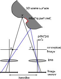
The most prominent, and the most detailed in this book, is the last mentioned of these. Here, depth is estimated by the geometric principle of triangulation, when the same scene point can be observed in two or more images. Figure 1.3 illustrates this principle in detail. Here, a rectilinear stereo rig is shown where the two cameras are side by side with the principal axes of their lenses parallel to each other. Note that the origin (or center) of each camera is the optical center of its lens and the baseline is defined as the distance between these two camera centers. Although the real image sensor is behind the lens, it is common practice to envisage and use a conceptual image position in front of the lens so that the image is the same orientation as the scene (i.e. not inverted top to bottom and left to right) and this position is shown in Fig. 1.3. The term triangulation comes from the fact that the scene point, X, can be reconstructed from the triangle18 formed by the baseline and the two coplanar vector directions defined by the left camera center to image point x and the right camera center to image point x . In fact, the depth of the scene is related to the disparity between left and right image correspondences. For closer objects, the disparity is greater, as illustrated by the blue lines in Fig. 1.3. It is clear from this figure that the

18This triangle defines an epipolar plane, which is discussed in Chap. 2.

12	R. Koch et al.

Fig. 1.3 A rectlinear stereo rig. Note the increased image disparity for the near scene point (blue) compared to the far scene point (black). The scene area marked in red can not be imaged by the right camera and is a ‘missing part’ in the reconstructed scene

scene surface colored red can not be observed by the right camera, in which case no 3D shape measurement can be made. This scene portion is sometimes referred to as a missing part and is the result of self-occlusion or occlusion by a different foreground object. Image correspondences are found by evaluating image similarities through image feature matching, either locally or globally over the entire image. Problems might occur if the image content does not hold sufficient information for unique correspondences, for example in smooth, textureless regions. Hence, a dense range estimation cannot be guaranteed and, particularly in man-made indoor scenarios, the resulting range images are often sparse. Algorithms, test scenarios and benchmarks for such systems may be found in the Middlebury database [42] and Chap. 2 in this book will discuss these approaches in detail. Note that many stereo rigs turn the cameras towards each other so that they are verged, which increases the overlap between the fields of view of the camera and increases the scene volume over which 3D reconstructions can be made. Such a system is shown in Fig. 1.4.

1.4.2 Active 3D Imaging

Active 3D imaging avoids some of the difficulties of passive techniques by introducing controlled additional information, usually controlled lighting or other electromagnetic radiation, such as infrared. Active stereo systems, for example, have the same underlying triangulation geometry as the above-mentioned passive stereo systems, but they exchange one camera by a projector, which projects a spot or a stripe, or a patterned area that does not repeat itself within some local neighborhood. This latter type of non-scanned system is called a structured light projection. Advances in optoelectronics for the generation of structured light patterns and other

1 Introduction

13

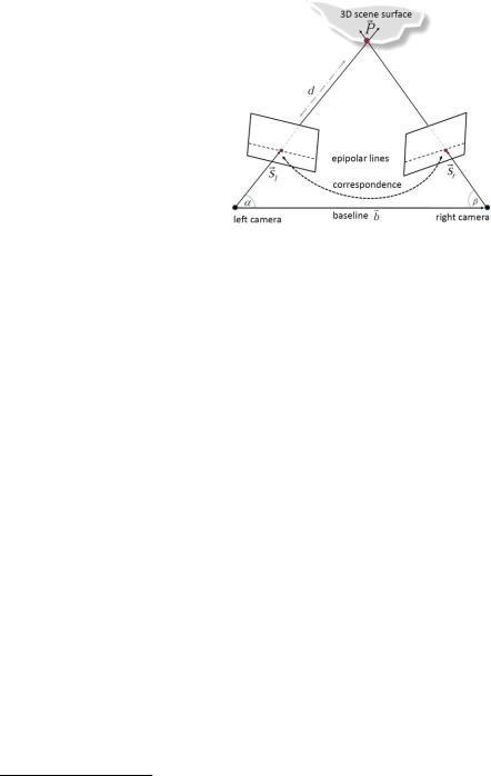
Fig. 1.4 A verged stereo system. Note that this diagram uses a simplified diagrammatic structure seen in much of the literature where only camera centers and conceptual image planes are shown. The intersection of the epipolar plane with the (image) planes defines a pair of epipolar lines. This is discussed in detail in Chap. 2. Figure reprinted from [29] with permission

illumination, accurate mechanical laser scanning control, and high resolution, high sensitivity image sensors have all had their impact on advancing the performance of active 3D imaging.

Note that, in structured light systems, all of the image feature shift that occurs due to depth variations, which causes a change in disparity, appears in the sensor’s one camera, because the projected image pattern is fixed. (Contrast this with a passive binocular stereo system, where the disparity change, in general, is manifested as feature movement across two images.) The projection of a pattern means that smooth, textureless areas of the scene are no longer problematic, allowing dense, uniform reconstructions and the correspondence problem is reduced to finding the known projected pattern. (In the case of a projected spot, the correspondence problem is removed altogether.) In general, the computational burden for generating active range triangulations is relatively light, the resulting range images are mostly dense and reliable, and they can be acquired quickly.

An example of such systems are coded light projectors that use either a timeseries of codes or color codes [8]. A recent example of a successful projection system is the Kinect-camera19 that projects an infrared dot pattern and is able to recover dense range images up to several meters distance at 30 frames per second (fps). One problem with all triangulation-based systems, passive and active, is that depth accuracy depends on the triangulation angle, which means that a large baseline is desirable. On the other hand, with a large baseline, the ‘missing parts’ problem described above is exacerbated, yielding unseen, occluded regions at object boundaries. This is unfortunate, since precise object boundary estimation is important for geometric reconstruction.

An alternative class of active range sensors that mitigates the occlusion problem are coaxial sensors, which exploit the time-of-flight principle. Here, light is emitted from a light source that is positioned in line with the optical axis of the receiving sensor (for example a camera or photo-diode) and is reflected from the object sur-

19Kinect is a trademark of Microsoft.