ATOMATIC CONTROL LABS

THE FIRST ORDER DYNAMIC SYSTEMS

Laboratory work No. 3

Objectives: to get acquinted with the first order dynamic systems and learn to analyze their characteristics in time and frequency domain.

Task:

1.Elaborate the mathematical modul of the system, indicated by teacher.

2.Expand elaborated model to series connection of the first order systems, if it is neccesary.

3.According to differential equations plot step responses and frequency responses.

4.Check results with Matlab software.

Theoretical part

The simplest transfer function is described by equation:

y Ku;

(1)

where: K is gain of the system.

Time domain analysis of Eq. (1) shows, that unit step response will have same shape as unit step 1(t), but its amplitude will increase by K times.

yp K1(t).

(2)

Plot of unit step 1(t) and response y is shown in Fig. 4. Transfer function of this system is:

41

GP K.					(3)
Frequency response of the system G j K 0 j.
Plot G j is given in Fig. 5.
Bode plot of this function is calculated as:
L 20lg		G j		20lg K;	(4)

and does not depend on frequency. Bode plot L is shown in Fig. 6. The phase angle of proportional system:

	tan 1	Im G j	tan 1 0 0;	(5)
		ReG j

is horizontal straight, shown in Fig. 7.

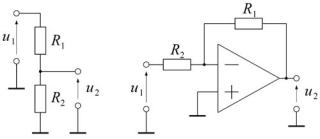
The simplest electrical examples of propotional system are shown in Fig. 1 a – voltage divider and Fig. 1 b – amplifier.

Fig.1. Example of projectional system

Output voltage U2 of voltage divider, shown in Fig. 1 a is calculated.

	u2			R2	u1.	(6)
			R1	R2
		42

Gain of the system depends on resistances R1 and R2 and changes in the range 0 K 1.

The system with operational amplifier gives posibility to change output voltage. For the ideal operational amplifier can be applied principle of virtual ground which gives:

u1	u2 ; u	2		R1	u .	(7)
R2	R1			R2	1

Therefore, varying ratio of R1R2 gives posibility to change

gain in wide range.

The propotional system has no inertic, nevertheless all real systems have that. Therefore propotional system is idealized real system. As example the real oscillograme of the operational amplifier, shown in Fig. 2, corresponding to the step response of amplifier, shown in Fig. 1 a.

In the circuit was used operational amplifier LM 741 and resistances R1 R2 10 kΩ.

Fig. 2. Impulse response of amplifier

The upper curve in Fig. 2 corresponds to input signal and lower curve corresponds to impulse response of amplifier. According to expression (7), gain K 1, therefore the inverted output signal is

43

shown in Fig. 2 to facilitate comparison of output and input signals. The amplifier was supplied by 10 kHz rectangular impulses. The

output signal has the front shape with slope sitting time of impulse response is about 10 s , which depends on inertic of operational

amplifier.

The integrating circuit. It is described as:

t			dy
y KI udt y0	;			KI u;	(8)
0			dt

where: KI – coefficient, y0 – initial value of output signal. Step response of integrating systems is:

t
yI KI	1(0)dt y0	KI t y0.	(9)
0

Expression (9) describes straight, which in Fig. 4 is marked by

y1 .

Assuming y0 0 and applying for Eq. (8) Laplace transform, the transfer function of integrating system is:

Y s	KI	U s ;		GI	KI	.
	s				s

Frequency response of integrator is:

GI ( j ) KI j KI . j

(10)

(11)

Expression (11) indicates the linear frequency response. Straight line begins at the point GI 0 j j and ends at the

point GI j 0 . Polar plot of integrating system is shown in Fig. 5. Bode plot of integrating circuit is calculated as:

L

( ) 20lg

G

( j )

20lg

KI

20lg K

I

20lg

.

(12)

I

I

44

Expression (12) is description of straight line. Increasing the frequency 10 times yields:

LI (10 ) 20lg KI 20lg10 20lg KI 20lg 20 (13) LI ( ) 20.

Comparison of (12) and (13) expressions show the reduction of integrating system magnitude by 20 dB/dec .

Frequency 0 , at which magnitude LI 0 0 , is called intersection frequency and calculated as:

20lg KI 20lg 0 0;

0 KI .

(14)

Bode plot of integrating system is shown in Fig. 6. Intersection frequency is 0 KI , and the slope of characteristic is equal to

20 dB/dec .

Semilog dependence phase ange versus frequency is calculated

as:

I arctan	ImGI j	arctan	K	I	/	90 .	(15)
	ReGI j			0

(15) shows, that output signal phase angle does not depend on frequency and is equal to -90 °. Graphically I is shown in Fig.

7.

The practical examples of integrating circuits are shown in Fig. 3.

45

Fig. 3. Examples of integrating systems

Mechanical system, shown in Fig. 3 a, is composed by the body of mass m, lying on the support. If the friction force between the body and surface, the dynamics of the system is described by the

second Newton‘s Law:
	m	dv		(16)
		dt	F;
where:
	F is force, acting the body, v is speed of the body.

If the movement is one dimensional, i.e. along x axis, the vec-

tor equation (16) can be replaced by projections of vectors:

m dvx

F ;

dvx

1

F

(17).

m

dt

x

dt

x

Assuming system input and output signals correspondingly

u F ;

y v

x

and

K

I

m 1 , the expression (17) becomes similar to

x

integrating system equation (8).

At analysis of circuit in Fig. 3 b it is convenient to apply virtual ground principle:

u1

i ;

u1

C

du2

;

du2

u1

. (18)

R

R

C R

2

1

dt

dt

1

1

1

1

46

Again, if the system output and input signals correspondingly

are u u ,	y u and	K	I		1	, the equation (18), describing the
1	e				C1R1

system, coincides with that of integrating system (8).

Many systems, having inertia, are described in time domain by the first order differential equation:

	a dy	a y b u.				(19)
	1 dt	0		0
	Denoting K A		b0	and T	a1	, the first order system is re-
			a0		a0
	written in this way:
	T dy	y KAu;				(20)
	dt

where: K A is the first order system gain and T is time con-

stant.

The general solution of homogenous system, in the engineering called as free movement, has the form:

y		C	exp			t		;	(21)
	h
		1
						T

where: C1 is integrating constant, calculated from initial con-

ditions, t is time.

Solution of Eq. 20 is equal to sum of solutions of general solution and solution of non-homogenic solution, which depends on input signal u. If the input signal is unit step and boundary conditions are assumed y 0 0 and y KA , then solution of Eq. (20) is:

y		K	1 exp			t	.	(22)
	A
			A
						T
			47

Unit step response of the first order system is plotted in Fig. 4 according to expression (22).

Fig. 4. Unit step responses of proportional (P), integrating (I) and first order system (A)

Figure 4 shows that unit response of first order system exponentially approaches to steady-state value K A . The settling time ts is

called the time, after which the response differs from steady-state value by assumed ε value. If it assumed that 5 %, then ts 3T .

For 2 %, settling time ts 4T .

The first order system transfer function is:

	GA s	KA		.	(23)
		Ts	1

Frequency response is calculated by replacing s with jω in transfer function (23):

	GA j	KA		KA			1 Tj	.	(24)
		Tj 1			1		T 2

Designating a T gives real and imaginary parts of frequency response in the form:

48

x Re G j

K A

; y Im G j

K

a

. (25)

1

a2

A 1 a2

From Eq. (25) is evident that:

a2

KA

1;

(26)

x

then:

KA

1

KA

y KA

x

x

1.

(27)

KA

x

x

Raising both sides of Eq. (27) in square and assuming thatx 0 : y 0 , yields:

	2		2			2		2		KA		KA 2			KA 2
y		KA x x		;	y		x		2		x						;	(28)
										2		2			2
	0;
y
						0.
					y

Finally, Eq. (28) can be rewritten as:

				K	A	2		K	A	2
	y2	x									(29)
				2				2
										.
	y 0.
	The first equation of the set (29) describes the circle with cen-
	ter coordinates		x0 0, KA					2		and radius	R KA 2 . The second

unequality shows, that the characteristic is situated in below horizontal axis. Therefore in general way polar plot of first order system is halfcircle, shown in Fig. 5.

49

Fig. 5. Polar plots of proportional (P), integrating (I) and first order system (A)

Figure 5 shows that the first order system frequency response

GA begins and ends on the real axis. Polar plot initial coordinates are x0 KA ,0 and finishing coordinates x 0,0 . The plot has the third characteristic point with coordinates x KA 2, KA 2 . It corresponds to frequency 1T .

Magnitude of frequency response is calculated from expression (24):

GA j

K

A

1 T 2

.

(30)

1 T 2

It is expressed in decibels:

K

A

1 T 2

L

A

20lg

G

A

j

20lg

. (31)

1

T

2

Simple program can be made to plot the expression (31), but design of controllers uses asymptotic diagrams, made from the straight lines, asymptotically approaching to actual diagram. Asymptotic, or corner Bode plot is analysed in the range of low and high

50