Fundamentals Of Wireless Communication

78	Point-to-point communication

Figure 3.12 (a) In the 1 × 2 channel, the signal space is one-dimensional, spanned by h. (b) In the 2 × 2 channel, the signal space is two-dimensional, spanned by h1 and h2.

In Section 2.2.3 we have defined the degrees of freedom of a channel as the dimension of the received signal space. In a channel with two transmit and a single receive antenna, this is equal to one for every symbol time. The repetition scheme utilizes only half a degree of freedom per symbol time, while the Alamouti scheme utilizes all of it.

With L receive, but a single transmit antenna, the received signal lies in an L-dimensional vector space, but it does not span the full space. To see this explicitly, consider the channel model from (3.69) (suppressing the symbol time index m):

y = hx + w

(3.89)

where y = y1 yL t h = h1 hL t and w = w1 wL t. The signal of interest, hx, lies in a one-dimensional space.11 Thus, we conclude that

the degrees of freedom of a multiple receive, single transmit antenna channel is still 1 per symbol time.

But in a 2 × 2 channel, there are potentially two degrees of freedom per symbol time. To see this, we can write the channel as

y = h1x1 + h2x2 + w

(3.90)

where xj and hj are the transmitted symbol and the vector of channel gains from transmit antenna j respectively, and y = y1 y2 t and w = w1 w2 t are the vectors of received signals and 0 N0 noise respectively. As long as h1 and h2 are linearly independent, the signal space dimension is 2: the signal from transmit antenna j arrives in its own direction hj , and with two receive antennas, the receiver can distinguish between the two signals. Compared to a 2 × 1 channel, there is an additional degree of freedom coming from space. Figure 3.12 summarizes the situation.

	h
			h1	x1		h2
	x				x2

(a)

(b)

11 This is why the scalar h / h y is a sufficient statistic to detect x (cf. (3.33)).

79	3.3 Antenna diversity

Spatial multiplexing

Now we see that neither the repetition scheme nor the Alamouti scheme utilizes all the degrees of freedom in a 2 × 2 channel. A very simple scheme that does is the following: transmit independent uncoded symbols over the different antennas as well as over the different symbol times. This is an example of a spatial multiplexing scheme: independent data streams are multiplexed in space. (It is also called V-BLAST in the literature.) To analyze the performance of this scheme, we extend the derivation of the pairwise error probability bound (3.85) from a single receive antenna to multiple receive antennas. Exercise 3.19 shows that with nr receive antennas, the corresponding bound on the probability of confusing codeword XB with codeword XA is

			L			1			nr
			$ +
XA	→	XB	≤							(3.91)
				1 1 SNR 2			/4
			=

where are the singular values of the codeword difference XA − XB. This bound holds for space-time codes of general block lengths. Our specific scheme does not code across time and is thus “space-only”. The block

length is 1, the codewords are two-dimensional vectors x1 x2							and the bound
simplifies to
	1					2
	x1 → x2 ≤
			1 + SNR x1 − x2 2/4
	16
	≤						(3.92)
		SNR2 x1 − x2 4

The exponent of the SNR factor is the diversity gain: the spatial multiplexing scheme achieves a diversity gain of 2. Since there is no coding across the transmit antennas, it is clear that no transmit diversity can be exploited; thus the diversity comes entirely from the dual receive antennas. The factor x1 − x2 4 plays a role analogous to the determinant det XA −XBXA − XB in determining the coding gain (cf. (3.86)).

Compared to the Alamouti scheme, we see that V-BLAST has a smaller diversity gain (2 compared to 4). On the other hand, the full use of the spatial degrees of freedom should allow a more efficient packing of bits, resulting in a better coding gain. To see this concretely, suppose we use BPSK symbols in the spatial multiplexing scheme to deliver 2 bits/s/Hz. Assuming that the average transmit energy per symbol time is normalized to be 1 as before, we can use (3.92) to explicitly calculate a bound on the worst-case pairwise error probability:

maxi j xi → xj ≤ 4 · SNR−2	(3.93)
=

80	Point-to-point communication

On the other hand, the corresponding bound for the Alamouti scheme using 4-PAM symbols to deliver the same 2 bits/s/Hz can be calculated from (3.86) to be

maxi j xi → xj ≤ 1600 · SNR−4	(3.94)
=

We see that indeed the bound for the Alamouti scheme has a much poorer constant before the factor that decays with SNR.

We can draw two lessons from the V-BLAST scheme. First, we see a new role for multiple antennas: in addition to diversity, they can also provide additional degrees of freedom for communication. This is in a sense a more powerful view of multiple antennas, one that will be further explored in Chapter 7. Second, the scheme also reveals limitations in our performance analysis framework for space-time codes. In the earlier sections, our approach has always been to seek schemes which extract the maximum diversity from the channel and then compare them on the basis of the coding gain, which is a function of how efficiently the schemes utilize the available degrees of freedom. This approach falls short in comparing V-BLAST and the Alamouti scheme for the 2 × 2 channel: V-BLAST has poorer diversity than the Alamouti scheme but is more efficient in exploiting the spatial degrees of freedom, resulting in a better coding gain. A more powerful framework combining the two performance measures into a unified metric is needed; this is one of the main subjects of Chapter 9. There we will also address the issue of what it means by an optimal scheme and whether it is possible to find a scheme which achieves the full diversity and the full degrees of freedom of the channel.

Low-complexity detection: the decorrelator

One advantage of the Alamouti scheme is its low-complexity ML receiver: the decoding decouples into two orthogonal single-symbol detection problems. ML detection of V-BLAST does not enjoy the same advantage: joint detection of the two symbols is required. The complexity grows exponentially with the number of antennas. A natural question to ask is: what performance can suboptimal single-symbol detectors achieve? We will study MIMO receiver architectures in depth in Chapters 7 and 9, but here we will give an example of a simple detector, the decorrelator, and analyze its performance in the 2 × 2 channel.

To motivate the definition of this detector, let us rewrite the channel (3.90) in matrix form:

y = Hx + w

(3.95)

where H = h1 h2 is the channel matrix. The input x = x1 x2 t is composed of two independent symbols x1 x2. To decouple the detection of the two symbols, one idea is to invert the effect of the channel:

y˜ = H−1y = x + H−1w = x + w˜

(3.96)

81	3.3 Antenna diversity

and detect each of the symbols separately. This is in general suboptimal compared to joint ML detection, since the noise samples w˜ 1 and w˜ 2 are correlated. How much performance do we lose?

Let us focus on the detection of the symbol x1 from transmit antenna 1. By direct computation, the variance of the noise w˜ 1 is

	h22 2 + h21 2	N0	(3.97)
	h11h22 − h21h12 2

Hence, we can rewrite the first component of the vector equation in (3.96) as

y˜1 = x1 + h22 2 + h21 2 z1 (3.98)h11h22 − h21h12

where z1 0 N0 , the scaled version of w˜ 1, is independent of x1. Equivalently, the scaled output can be written as

	y			h11h22 − h21h12			y
	1		=		h22 2 + h21 2		˜1
		= 2h1 x1 + z1						(3.99)
where
hi1			1			hi2
hi = hi2	i =					−hi1		i = 1 2 (3.100)
				hi2 2 + hi1 2

Geometrically, one can interpret hj as the “direction” of the signal from transmit antenna j and j as the direction orthogonal to hj . Equation (3.99) says that when demodulating the symbol from antenna 1, channel inversion eliminates the interference from transmit antenna 2 by projecting the received signal y in the direction orthogonal to h2 (Figure 3.13). The signal part is2h1 x1. The scalar gain 2h1 is circular symmetric Gaussian, being the projection of a two-dimensional i.i.d. circular symmetric Gaussian random vector (h1) onto an independent unit vector ( 2) (cf. (A.22) in Appendix A). The scalar channel (3.99) is therefore Rayleigh faded like a 1 ×1 channel and has only unit diversity. Note that if there were no interference from antenna 2, the diversity gain would have been 2: the norm h1 2 of the entire vector h1 has to be small for poor reception of x1. However, here, the component of h1 perpendicular to h2 being small already wreacks havoc; this is the price paid for nulling out the interference from antenna 2. In contrast, the ML detector, by jointly detecting the two symbols, retains the diversity gain of 2.

We have discussed V-BLAST in the context of a point-to-point link with two transmit antennas. But since there is no coding across the antennas, we can equally think of the two transmit antennas as two distinct users each with a single antenna. In the multiuser context, the receiver described above is sometimes called the interference nuller, zero-forcing receiver or

82	Point-to-point communication

Figure 3.13 Demodulation of x1: the received vector y is projected onto the direction2 orthogonal to h2. The effective channel for x1 is in deep fade whenever the projection of h1 onto 2 is small.

y2
y	φ2
h2
	h1
	y1

the decorrelator. It nulls out the effect of the other user (interferer) while demodulating the symbol of one user. Using this receiver, we see that dual receive antennas can perform one of two functions in a wireless system: they can either provide a two-fold diversity gain in a point-to-point link when there is no interference, or they can be used to null out the effect of an interfering user but provide no diversity gain more than 1. But they cannot do both. This is however not an intrinsic limitation of the channel but rather a limitation of the decorrelator; by performing joint ML detection instead, the two users can in fact be simultaneously supported with a two-fold diversity gain each.

Summary 3.2 2 × 2 MIMO schemes

The performance of the various schemes for the 2 × 2 channel is summarized below.

		Degrees of freedom utilized
	Diversity gain	per symbol time
Repetition	4	1/2
Alamouti	4	1
V-BLAST (ML)	2	2
V-BLAST (nulling)	1	2
Channel itself	4	2

83	3.4 Frequency diversity

3.4 Frequency diversity

3.4.1 Basic concept

So far we have focused on narrowband flat fading channels. These channels are modeled by a single-tap filter, as most of the multipaths arrive during one symbol time. In wideband channels, however, the transmitted signal arrives over multiple symbol times and the multipaths can be resolved at the receiver. The frequency response is no longer flat, i.e., the transmission bandwidth W is greater than the coherence bandwidth Wc of the channel. This provides another form of diversity: frequency.

We begin with the discrete-time baseband model of the wireless channel in Section 2.2. Recalling (2.35) and (2.38), the sampled output y m can be written as

y m = h m x m − + w m (3.101)

Here h m denotes the th channel filter tap at time m. To understand the concept of frequency diversity in the simplest setting, consider first the oneshot communication situation when one symbol x0 is sent at time 0, and no symbols are transmitted after that. The receiver observes

y = h x0 + w

= 0 1 2

(3.102)

If we assume that the channel response has a finite number of taps L, then the delayed replicas of the signal are providing L branches of diversity in detecting x0 , since the tap gains h are assumed to be independent. This diversity is achieved by the ability of resolving the multipaths at the receiver due to the wideband nature of the channel, and is thus called frequency diversity.

A simple communication scheme can be built on the above idea by sending an information symbol every L symbol times. The maximal diversity gain of L can be achieved, but the problem with this scheme is that it is very wasteful of degrees of freedom: only one symbol can be transmitted every delay spread. This scheme can actually be thought of as analogous to the repetition codes used for both time and spatial diversity, where one information symbol is repeated L times. In this setting, once one tries to transmit symbols more frequently, inter-symbol interference (ISI) occurs: the delayed replicas of previous symbols interfere with the current symbol. The problem is then how to deal with the ISI while at the same time exploiting the inherent frequency diversity in the channel. Broadly speaking, there are three common approaches:

•Single-carrier systems with equalization By using linear and non-linear processing at the receiver, ISI can be mitigated to some extent. Optimal ML detection of the transmitted symbols can be implemented using the Viterbi algorithm. However, the complexity of the Viterbi algorithm grows

84	Point-to-point communication

exponentially with the number of taps, and it is typically used only when the number of significant taps is small. Alternatively, linear equalizers attempt to detect the current symbol while linearly suppressing the interference from the other symbols, and they have lower complexity.

•Direct-sequence spread-spectrum In this method, information symbols are modulated by a pseudonoise sequence and transmitted over a bandwidth W much larger than the data rate. Because the symbol rate is very low, ISI is small, simplifying the receiver structure significantly. Although this leads to an inefficient utilization of the total degrees of freedom in the system from the perspective of one user, this scheme allows multiple users to share the total degrees of freedom, with users appearing as pseudonoise to each other.

•Multi-carrier systems Here, transmit precoding is performed to convert the ISI channel into a set of non-interfering, orthogonal sub-carriers, each experiencing narrowband flat fading. Diversity can be obtained by coding across the symbols in different sub-carriers. This method is also called Discrete Multi-Tone (DMT) or Orthogonal Frequency Division Multiplexing (OFDM). Frequency-hop spread-spectrum can be viewed as a special case where one carrier is used at a time.

For example, GSM is a single-carrier system, IS-95 CDMA and IEEE 802.11b (a wireless LAN standard) are based on direct-sequence spreadspectrum, and IEEE 802.11a is a multi-carrier system,

Below we study these three approaches in turn. An important conceptual point is that, while frequency diversity is something intrinsic in a wideband channel, the presence of ISI is not, as it depends on the modulation technique used. For example, under OFDM, there is no ISI, but sub-carriers that are separated by more than the coherence bandwidth fade more or less independently and hence frequency diversity is still present.

Narrowband systems typically operate in a relatively high SNR regime. In contrast, the energy is spread across many degrees of freedom in many wideband systems, and the impact of the channel uncertainty on the ability of the receiver to extract the inherent diversity in frequency-selective channels becomes more pronounced. This point will be discussed in Section 3.5, but in the present section, we assume that the receiver has a perfect estimate of the channel.

3.4.2 Single-carrier with ISI equalization

Single-carrier with ISI equalization is the classic approach to communication over frequency-selective channels, and has been used in wireless as well as wireline applications such as voiceband modems. Much work has been done in this area but here we focus on the diversity aspects.

Starting at time 1, a sequence of uncoded independent symbols x1 x2 is transmitted over the frequency-selective channel (3.101).

85	3.4 Frequency diversity

Assuming that the channel taps do not vary over these N symbol times, the received symbol at time m is

	L−1
y m =
	h x m − + w m	(3.103)

=0

where x m = 0 for m < 1. For simplicity, we assume here that the taps h are i.i.d. Rayleigh with equal variance 1/L, but the discussion below holds more generally (see Exercise 3.25).

We want to detect each of the transmitted symbols from the received signal. The process of extracting the symbols from the received signal is called equalization. In contrast to the simple scheme in the previous section where a symbol is sent every L symbol times, here a symbol is sent every symbol time and hence there is significant ISI. Can we still get the maximum diversity gain of L?

Frequency-selective channel viewed as a MISO channel

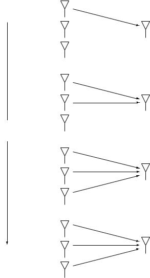
To analyze this problem, it is insightful to transform the frequency-selective channel into a flat fading MISO channel with L transmit antennas and a single receive antenna and channel gains h0 hL−1. Consider the following transmission scheme on the MISO channel: at time 1, the symbol x1 is transmitted on antenna 1 and the other antennas are silent. At time 2, x1 is transmitted at antenna 2, x2 is transmitted on antenna 1 and the other antennas remain silent. At time m, x m − is transmitted on antenna + 1, for = 0 L − 1. See Figure 3.14. The received symbol at time m in this MISO channel is precisely the same as that in the frequency-selective channel under consideration.

Once we transform the frequency-selective channel into a MISO channel, we can exploit the machinery developed in Section 3.3.2. First, it is clear that if we want to achieve full diversity on a symbol, say x N, we need to observe the received symbols up to time N +L−1. Over these symbol times, we can write the system in matrix form (as in (3.80)):

yt = h X + wt

(3.104)

where yt = y1 y N + L − 1 h = h0 hL−1 wt = w1

w N + L − 1 and the L by N + L − 1 space-time code matrix

x1

x2

·

·

·

x N

·

·

x N L

−

1

0

x1

x2

·

·

x N

+

2

·

·

x N + L

−

·

·

·

·

·

·

·

·

·

X =

(3.105)

0

0

x1

x2

·

·

·

·

·

·

·

·

·

0

0

x1

x2

x N

corresponds to the transmitted sequence x = x1 x N + L − 1 t.

86

Figure 3.14 The MISO scenario equivalent to the frequencyselective channel.

Point-to-point communication

x [1]

x [2]

x [1]

Increasing

time

x [3]

x [2]

x [3]

x [4]

x [3]

x [2]

h0

h0

h1

h0

h1

h2

h0

h1

h2

y[1]

y[2]

y[3]

y[4]

Error probability analysis

Consider the maximum likelihood detection of the sequence x based on the received vector y (MLSD). With MLSD, the pairwise error probability of confusing xA with xB, when xA is transmitted is, as in (3.85),

	L		1
xA → xB ≤	$ +					(3.106)
	=1	1 SNR 2		/4

where 2 are the eigenvalues of the matrix XA − XB XA − XB and SNR is the total received SNR per received symbol (summing over all paths). This

87	3.4 Frequency diversity

error probability decays like SNR−L whenever the difference matrix XA − XB is of rank L.

By a union bound argument, the probability of detecting the particular

symbol x N incorrectly is bounded by
xA → xB	(3.107)

xB xB N =xA N

summing over all the transmitted vectors xB which differ with xA in the N th symbol.12 To get full diversity, the difference matrix XA − XB must be full rank for every such vector xB (cf. (3.86)). Suppose m is the symbol time in which the vectors xA and xB first differ. Since they differ at least once within the first N symbol times, m ≤ N and the difference matrix is of the form

0	·		0
0		0 xA m − xB m
XA − XB = 0 · ·			·
	·	·
·	·	·	·
0	·	·	·

xA m	0	xB m	·	·	·
	·		·	·	·
	−		·	·	·
	·		·	·	·

·0 xA m − xB m ·

(3.108)

By inspection, all the rows in the difference matrix are linearly independent. Thus XA −XB is of full rank (i.e., the rank is equal to L). We can summarize:

Uncoded transmission combined with maximum likelihood sequence detection achieves full diversity on symbol x N using the observations up to time N + L − 1, i.e., a delay of L − 1 symbol times.

Compared to the scheme in which a symbol is transmitted every L symbol times, the same diversity gain of L is achieved and yet an independent symbol can be transmitted every symbol time. This translates into a significant “coding gain” (Exercise 3.26).

In the analysis here it was convenient to transform the frequency-selective channel into a MISO channel. However, we can turn the transformation around: if we transmit the space-time code of the form in (3.105) on a MISO channel, then we have converted the MISO channel into a frequency-selective

12Strictly speaking, the MLSD only minimizes the sequence error probability, not the symbol error probability. However, this is the standard detector implemented for ISI equalization via the Viterbi algorithm, to be discussed next. In any case, the symbol error probability performance of the MLSD serves as an upper bound to the optimal symbol error performance.