Fundamentals Of Wireless Communication

108 Point-to-point communication

measurement problem is the same as with a single receive antenna and does not become harder. The situation is similar in the time diversity scenario. In antenna diversity with L transmit antennas, the received energy per diversity path does decrease with the number of antennas used, but certainly we can restrict the number L to be the number of different channels that can be reliably learnt by the receiver.

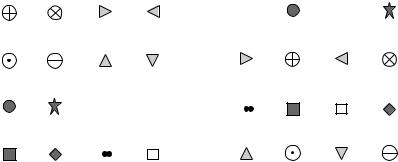
How about in OFDM systems with frequency diversity? Here, the designer has control over how many sub-carriers to spread the signal energy over. Thus, while the number of available diversity branches L may increase with the bandwidth, the signal energy can be restricted to a fixed number of subcarriers L < L over any one OFDM time block. Such communication can be restricted to concentrated time-frequency blocks and Figure 3.25 visualizes one such scheme (for L = 2), where the choice of the L sub-carriers is different for different OFDM blocks and is hopped over the entire bandwidth. Since the energy in each OFDM block is concentrated within a fixed number of sub-carriers at any one time, coherent reception is possible. On the other hand, the maximum diversity gain of L can still be achieved by coding across the sub-carriers within one OFDM block as well as across different blocks.

One possible drawback is that since the total power is only concentrated within a subset of sub-carriers, the total degrees of freedom available in the system are not utilized. This is certainly the case in the context of point-to- point communication; in a system with other users sharing the same bandwidth, however, the other degrees of freedom can be utilized by the other users and need not go wasted. In fact, one key advantage of OFDM over DS spread-spectrum is the ability to maintain orthogonality across multiple users in a multiple access scenario. We will return to this point in Chapter 4.

Figure 3.25 An illustration of a scheme that uses only a fixed part of the bandwidth at every time. Here, one small square denotes a single sub-carrier within one OFDM block. The time-axis indexes the different OFDM blocks; the frequency-axis indexes the different sub-carriers.

Frequency

Time

109	3.5 Impact of channel uncertainty

Chapter 3 The main plot

Baseline

We first looked at detection on a narrowband slow fading Rayleigh channel. Under both coherent and non-coherent detection, the error probability behaves like

pe ≈ SNR−1

(3.157)

at high SNR. In contrast, the error probability decreases exponentially with the SNR in the AWGN channel. The typical error event for the fading channel is due to the channel being in deep fade rather than the Gaussian noise being large.

Diversity

Diversity was presented as an effective approach to improve performance drastically by providing redundancy across independently faded branches. Three modes of diversity were considered:

•time – the interleaving of coded symbols over different coherence time periods;

•space – the use of multiple transmit and/or receive antennas;

•frequency – the use of a bandwidth greater than the coherence bandwidth of the channel.

In all cases, a simple scheme that repeats the information symbol across the multiple branches achieves full diversity. With L i.i.d. Rayleigh branches of diversity, the error probability behaves like

pe ≈ c · SNR−L

(3.158)

at high SNR.

Examples of repetition schemes:

•repeating the same symbol over different coherence periods;

•repeating the same symbol over different transmit antennas one at a time;

•repeating the same symbol across OFDM sub-carriers in different coherence bands;

•transmitting a symbol once every delay spread in a frequency-selective channel so that multiple delayed replicas of the symbol are received without interference.

Code design and degrees of freedom

More sophisticated schemes cannot achieve higher diversity gain but can provide a coding gain by improving the constant c in (3.158). This is

110	Point-to-point communication

achieved by utilizing the available degrees of freedom better than in the repetition schemes.

Examples:

•rotation and permutation codes for time diversity and for frequency diversity in OFDM;

•Alamouti scheme for transmit diversity;

•uncoded transmission at symbol rate in a frequency-selective channel with ISI equalization.

Criteria to design schemes with good coding gain were derived for the different scenarios by using the union bound (based on pairwise error probabilities) on the actual error probability:

•product distance between codewords for time diversity;

•determinant criterion for space-time codes.

Channel uncertainty

The impact of channel uncertainty is significant in scenarios where there are many diversity branches but only a small fraction of signal energy is received along each branch. Direct-sequence spread-spectrum is a prime example.

The gap between coherent and non-coherent schemes is very significant in this regime. Non-coherent schemes do not work well as they cannot combine the signals along each branch effectively.

Accurate channel estimation is crucial. Given the amount of transmit power devoted to channel estimation, the efficacy of detection performance depends on the key parameter SNRest, the received SNR per coherence time per diversity branch. If SNRest 0 dB, then detection performance is near coherent. If SNRest 0 dB, then effective combining is impossible.

Impact of channel uncertainty can be ameliorated in some schemes where the transmit energy can be focused on smaller number of diversity branches. Effectively SNRest is increased. OFDM is an example.

3.6 Bibliographical notes

Reliable communication over fading channels has been studied since the 1960s. Improving the performance via diversity is also an old topic. Standard digital communication texts contain many formulas for the performance of coherent and non-coherent diversity combiners, which we have used liberally in this chapter (see Chapter 14 of Proakis [96], for example).

Early works recognizing the importance of the product distance criterion for improving the coding gain under Rayleigh fading are Wilson and Leung [144] and Divsalar

111 3.7 Exercises

and Simon [30], in the context of trellis-coded modulation. The rotation example is taken from Boutros and Viterbo [13]. Transmit antenna diversity was studied extensively in the late 1990s code design criteria were derived by Tarokh et al. [115] and by Guey et al. [55]; in particular, the determinant criterion is obtained in Tarokh et al. [115]. The delay diversity scheme was introduced by Seshadri and Winters [107]. The Alamouti scheme was introduced by Alamouti [3] and generalized to orthogonal designs by Tarokh et al. [117]. The diversity analysis of the decorrelator was performed by Winters et al. [145], in the context of a space-division multiple access system with multiple receive antennas.

The topic of equalization has been studied extensively and is covered comprehensively in standard textbooks on communication theory; for example, see the book by Barry et al. [4]. The Viterbi algorithm was introduced in [139]. The diversity analysis of MLSD is adopted from Grokop and Tse [54].

The OFDM approach to communicate over a wideband channel was first used in military systems in the 1950s and discussed in early papers in the 1960s by Chang [18] and Saltzberg [104]. Circular convolution and the DFT are classical undergraduate material in digital signal processing (Chapter 8, and Section 8.7.5, in particular, of [87]).

The spread-spectrum approach to harness frequency diversity has been well summarized by Viterbi [140]. The Rake receiver was designed by Price and Green [95]. The impact of channel uncertainty on the performance has been studied by various authors, including Médard and Gallager [85], Telatar and Tse [120] and Subramanian and Hajek [113].

3.7 Exercises

Exercise 3.1 Verify (3.19) and the high SNR approximation (3.21). Hint: Write the expression as a double integral and interchange the order of integration.

Exercise 3.2 In Section 3.1.2 we studied the performance of antipodal signaling under coherent detection over a Rayleigh fading channel. In particular, we saw that the error probability pe decreases like 1/SNR. In this question, we study a deeper characterization of the behavior of pe with increasing SNR.

1.A precise way of saying that pe decays like 1/SNR with increasing SNR is the following:

lim pe · SNR = c

SNR→

where c is a constant. Identify the value of c for the Rayleigh fading channel.

2.Now we want to test how robust the above result is with respect to the fading distribution. Let h be the channel gain, and suppose h 2 has an arbitrary continuous pdf f satisfying f 0 > 0. Does this give enough information to compute the high SNR error probability like in the previous part? If so, compute it. If not, specify what other information you need. Hint: You may need to interchange limit and integration in your calculations. You can assume that this can be done without worrying about making your argument rigorous.

3.Suppose now we have L independent branches of diversity with gains h1 hL, and h 2 having an arbitrary distribution as in the previous part. Is there enough

112	Point-to-point communication

information for you to find the high SNR performance of repetition coding and coherent combining? If so, compute it. If not, what other information do you need?

4.Using the result in the previous part or otherwise, compute the high SNR performance under Rician fading. How does the parameter affect the performance?

Exercise 3.3 This exercise shows how the high SNR slope of the probability of error (3.19) versus SNR curve can be obtained using a typical error event analysis, without the need for directly carrying out the integration.

Fix > 0 and define the -typical error events and − , where

= h h 2 < 1/SNR1−

1. By conditioning on the event , show that at high SNR

lim	log pe			≤ −		1	−
SNR→ log SNR
2. By conditioning on the event − , show that
lim	log pe			≥ −		1	+
SNR→ log SNR
3. Hence conclude that
lim		log pe						1
SNR→ log SNR = −

(3.159)

(3.160)

(3.161)

(3.162)

This says that the asymptotic slope of the error probability versus SNR plot (in dB/dB scale) is −1.

Exercise 3.4 In Section 3.1.2, we saw that there is a 4-dB energy loss when using 4-PAM on only the I channel rather than using QPSK on both the I and the Q channels, although both modulations convey two bits of information. Compute the corresponding loss when one wants to transmit k bits of information using 2k-PAM rather than 2k-QAM. You can assume k to be even. How does the loss depend on k?

Exercise 3.5 Consider the use of the differential BPSK scheme proposed in Section 3.1.3 for the Rayleigh flat fading channel.

1.Find a natural non-coherent scheme to detect u m based on y m − 1 and y m, assuming the channel is constant across the two symbol times. Your scheme does not have to be the ML detector.

2.Analyze the performance of your detector at high SNR. You may need to make some approximations. How does the high SNR performance of your detector compare to that of the coherent detector?

3.Repeat your analysis for differential QPSK.

Exercise 3.6 In this exercise we further study coherent detection in Rayleigh fading.

1.Verify Eq. (3.37).

2.Analyze the error probability performance of coherent detection of binary orthogonal signaling with L branches of diversity, under an i.i.d. Rayleigh fading assumption (i.e., verify Eq. (3.149)).

113 3.7 Exercises

Exercise 3.7 In this exercise, we study the performance of the rotated code in

Section 3.2.2.

1.Give an explicit expression for the exact pairwise error probability xA → xB in (3.49). Hint: The techniques from Exercise 3.1 will be useful here.

2.This pairwise error probability was upper bounded in (3.54). Show that the product of SNR and the difference between the upper bound and the actual pairwise error probability goes to zero with increasing SNR. In other words, the upper bound in (3.54) is tight up to the leading term in 1/SNR.

Exercise 3.8 In the text, we mainly use real symbols to simplify the notation. In practice, complex constellations are used (i.e., symbols are sent along both the I and Q components). The simplest complex constellation is QPSK: the constellation is a1 + j a1 − j a−1 − j a−1 + j .

1.Compute the error probability of QPSK detection for a Rayleigh fading channel with repetition coding over L branches of diversity. How does the performance compare to a scheme which uses only real symbols?

2.In Section 3.2.2, we developed a diversity scheme based on rotation of real symbols (thus using only the I channel). One can develop an analogous scheme for QPSK complex symbols, using a 2 ×2 complex unitary matrix instead. Find an analogous pairwise code-design criterion as in the real case.

3.Real orthonormal matrices are special cases of complex unitary matrices. Within the class of real orthonormal matrices, find the optimal rotation to maximize your criterion.

4.Find the optimal unitary matrix to maximize your criterion. (This may be difficult!)

Exercise 3.9 In Section 3.2.2, we rotate two BPSK symbols to demonstrate the possible improvement over repetition coding in a time diversity channel with two diversity paths. Continuing with the same model, now consider transmitting at a higher rate using a 2n-PAM constellation for each symbol. Consider rotating the resulting 2D constellation by a rotation matrix of the form in (3.46). Using the performance criterion of the minimum squared product distance, construct the optimal rotation matrix.

Exercise 3.10 In Section 3.2.2, we looked at the example of the rotation code to achieve time diversity (with the number of branches, L, equal to 2). In the text, we use real symbols and in Exercise 3.8 we extend to complex symbols. In the latter scenario, another coding scheme is the permutation code. Shown in Figure 3.26 are two 16QAM constellations. Each codeword in the permutation code for L = 2 is obtained by picking a pair of points, one from each constellation, which are represented by the same icon. The codeword is transmitted over two (complex) symbol times.

1.Why do you think this is called a permutation code?

2.What is the data rate of this code?

3.Compute the diversity gain and the minimum product distance for this code.

4.How does the performance of this code compare to the rotation code in Exercise 3.8, part (3), in terms of the transmit power required?

Exercise 3.11 In the text, we considered the use of rotation codes to obtain time diversity. Rotation codes are designed specifically for fading channels. Alternatively, one can use standard AWGN codes like binary linear block codes. This question looks at the diversity performance of such codes.

114	Point-to-point communication
Figure 3.26 A permutation	♣	♠
code.

♣ ♠

Consider a perfectly interleaved Rayleigh fading channel:

y = h x + w = 1 L

where h and w are i.i.d. 0 1 and 0 N0 random variables respectively. A L k binary linear block code is specified by a k by L generator matrix G whose entries are 0 or 1. k information bits form a k-dimensional binary-valued vector b which is mapped into the binary codeword c = Gtb of length L, which is then mapped into L BPSK symbols and transmitted over the fading channel.16 The receiver is assumed to have a perfect estimate of the channel gains h .

1.Compute a bound on the error probability of ML decoding in terms of the SNR and parameters of the code. Hence, compute the diversity gain in terms of code parameter(s).

2.Use your result in (1) to compute the diversity gain of the (3, 2) code with generator matrix:

G =	1	0	1		(3.163)
	0	1	1

How does the performance of this code compare to the rate 1/2 repetition code?

3.The ML decoding is also called soft decision decoding as it takes the entire received vector y and finds the transmitted codeword closest in Euclidean distance to it. Alternatively, a suboptimal but lower-complexity decoder uses hard decision decoding, which for each first makes a hard decision cˆ on the th transmitted

coded symbol based only on the corresponding received symbol y , and then finds the codeword that is closest in Hamming distance to cˆ. Compute the diversity gain

of this scheme in terms of basic parameters of the code. How does it compare to the diversity gain achieved by soft decision decoding? Compute the diversity gain of the code in part (2) under hard decision decoding.

4.Suppose now you still do hard decision decoding except that you are allowed to also declare an “erasure” on some of the transmitted symbols (i.e., you can refuse to make a hard decision on some of the symbols). Can you design a scheme that

16 Addition and multiplication are done in the binary field.

115	3.7 Exercises

yields a better diversity gain than the scheme in part (3)? Can you do as well as soft decision decoding? Justify your answers. Try your scheme out on the example in part (2). Hint: the trick is to figure out when to declare an erasure. You may want to start thinking of the problems in terms of the example in part (2). The typical error event view in Exercise 3.3 may also be useful here.

Exercise 3.12 In our study of diversity models (cf. (3.31)), we have modeled the L branches to have independent fading coefficients. Here we explore the impact of correlation between the L diversity branches. In the time diversity scenario, consider the correlated model: h1 hL are jointly circular symmetric complex Gaussian with zero mean and covariance Kh ( 0 Kh in our notation).

1.Redo the diversity calculations for repetition coding (Section 3.2.1) for this correlated channel model by calculating the rate of decay of error probability with SNR. What is the dependence of the asymptotic (in SNR) behavior of the typical

error event on the correlation Kh? You can answer this by characterizing the rate of decay of (3.42) at high SNR (as a function of Kh).

2.We arrived at the product distance code design criterion to harvest coding gain along with time diversity in Section 3.2.2. What is the analogous criterion for correlated channels? Hint: Jointly complex Gaussian random vectors are related

to i.i.d. complex Gaussian vectors via a linear transformation that depends on the covariance matrix.

3. For transmit diversity with independent fading across the transmit antennas, we have arrived at the generalized product distance code design criterion in Section 3.3.2. Calculate the code design criterion for the correlated fading channel here (the channel h in (3.80) is now 0 Kh ).

Exercise 3.13 The optimal coherent receiver for repetition coding with L branches of diversity is a maximal ratio combiner. For implementation reasons, a simpler receiver one often builds is a selection combiner. It does detection based on the received signal along the branch with the strongest gain only, and ignores the rest. For the i.i.d. Rayleigh fading model, analyze the high SNR performance of this scheme. How much of the inherent diversity gain can this scheme get? Quantify the performance loss from optimal combining. Hint: You may find the techniques developed in Exercise 3.2 useful for this problem.

Exercise 3.14 It is suggested that full diversity gain can be achieved over a Rayleigh faded MISO channel by simply transmitting the same symbol at each of the transmit antennas simultaneously. Is this correct?

Exercise 3.15 An L × 1 MISO channel can be converted into a time diversity channel with L diversity branches by simply transmitting over one antenna at a time.

1.In this way, any code designed for a time diversity channel with L diversity branches can be used for a MISO (multiple input single output) channel with L transmit antennas. If the code achieves k-fold diversity in the time diversity channel, how much diversity can it obtain in the MISO channel? What is the relationship between the minimum product distance metric of the code when viewed as a time diversity code and its minimum determinant metric when viewed as a transmit diversity code?

116	Point-to-point communication

2.Using this transformation, the rotation code can be used as a transmit diversity scheme. Compare the performance of this code and the Alamouti scheme in a 2 ×1 Rayleigh fading channel, using BPSK symbols. Which one is better? How about using QPSK symbols?

3.Use the permutation code (cf. Figure 3.26) from Exercise 3.10 on the 2×1 Rayleigh fading channel and compare (via a numerical simulation) its performance with the Alamouti scheme using QPSK symbols (so the rate is the same in both the schemes).

Exercise 3.16 In this exercise, we derive some properties a code construction must satisfy to mimic the Alamouti scheme behavior for more than two transmit antennas. Consider communication over n time slots on the L transmit antenna channel (cf. (3.80)):

yt = h X + wt

(3.164)

Here X is the L × n space-time code. Over n time slots, we want to communicate L independent constellation symbols, d1 dL; the space-time code X is a deterministic function of these symbols.

1.Consider the following property for every channel realization h and space-time codeword X

h X t = Ad

(3.165)

Here we have written d = d1 dL t and A = a1 aL , a matrix with orthogonal columns. The vector d depends solely on the codeword X and the

matrix A depends solely on the channel h. Show that, if the space-time codeword X satisfies the property in (3.165), the joint receiver to detect d separates into individual linear receivers, each separately detecting d1 dL.

2.We would like the effective channel (after the linear receiver) to provide each symbol dm (m = 1 L) with full diversity. Show that, if we impose the condition that

am = h m = 1 L

(3.166)

then each data symbol dm has full diversity.

3.Show that a space-time code X satisfying (3.165) (the linear receiver property) and (3.166) (the full diversity property) must be of the form

XX = d 2IL

(3.167)

i.e., the columns of X must be orthogonal. Such an X is called an orthogonal design. Indeed, we observe that the codeword X in the Alamouti scheme (cf. (3.77)) is an orthogonal design with L = n = 2.

Exercise 3.17 This exercise is a sequel to Exercise 3.16. It turns out that if we require n = L, then for L > 2 there are no orthogonal designs. (This result is proved in Theorem 5.4.2 in [117].) If we settle for n > L then orthogonal designs exist for

117 3.7 Exercises

L > 2. In particular, Theorem 5.5.2 of [117] constructs orthogonal designs for all L and n ≥ 2L. This does not preclude the existence of orthogonal designs with rate larger than 0.5. A reading exercise is to study [117] where orthogonal designs with rate larger than 0.5 are constructed.

Exercise 3.18 The pairwise error probability analysis for the i.i.d. Rayleigh fading channel has led us to the product distance (for time diversity) and generalized product distance (for transmit diversity) code design criteria. Extend this analysis for the i.i.d. Rician fading channel.

1.Does the diversity order change for repetition coding over a time diversity channel with the L branches i.i.d. Rician distributed?

2.What is the new code design criterion, analogous to product distance, based on the pairwise error probability analysis?

Exercise 3.19 In this exercise we study the performance of space-time codes (the subject of Section 3.3.2) in the presence of multiple receive antennas.

1.Derive, as an extension of (3.83), the pairwise error probability for space-time codes with nr receive antennas.

2.Assuming that the channel matrix has i.i.d. Rayleigh components, derive, as an extension of (3.86), a simple upper bound for the pairwise error probability.

3.Conclude that the code design criterion remains unchanged with multiple receive antennas.

Exercise 3.20 We have studied the performance of the Alamouti scheme in a channel with two transmit and one receive antenna. Suppose now we have an additional receive antenna. Derive the ML detector for the symbols based on the received signals at both receive antennas. Show that the scheme effectively provides two independent scalar channels. What is the gain of each of the channels?

Exercise 3.21 In this exercise we study some expressions for error probabilities that arise in Section 3.3.3.

1.Verify Eqs. (3.93) and (3.94). In which SNR range is (3.93) smaller than (3.94)?

2.Repeat the derivation of (3.93) and (3.94) for a general target rate of R bits/s/Hz (suppose that R is an integer). How does the SNR range in which the spatial multiplexing scheme performs better depend on R?

Exercise 3.22 In Section 3.3.3, the performance comparison between the spatial multiplexing scheme and the Alamouti scheme is done for PAM symbols. Extend the comparison to QAM symbols with the target data rate R bits/s/Hz (suppose that R ≥ 4 is an even integer).

Exercise 3.23 In the text, we have developed code design criteria for pure time diversity and pure spatial diversity scenarios. In some wireless systems, one can get both time and spatial diversity simultaneously, and we want to develop a code design criterion for that. More specifically, consider a channel with L transmit antennas and 1 receive antenna. The channel remains constant over blocks of k symbol times, but changes to an independent realization every k symbols (as a result of interleaving, say). The channel is assumed to be independent across antennas. All channel gains are Rayleigh distributed.