Fundamentals Of Wireless Communication

198	Capacity of wireless channels

Figure 5.18 Effect of the fading gains on codes for the parallel channel. Here there are L= 2 sub-channels and each axis represents Tc dimensions within a sub-channel. (a) Coding across the sub-channels. The code works as long as the volume of the ellipsoid is big enough. This requires good codeword separation in both the sub-channels. (b) Separate, non-adaptive code for each sub-channel. Shrinking of one of the axes is enough to cause confusion between the codewords.

Extensions

Channel	Channel
fade	fade

Reliable communication	Noise spheres overlap
(a)	(b)

(here Tc = 1 symbol and L = 2 sub-channels). More generally, the code design criterion of maximizing the product distance for all pairs of codewords naturally favors codes that satisfy this property. Coding over long blocks affords a larger coding gain; information theory guarantees the existence of codes with large enough coding gain to achieve the outage probability in (5.83).

To achieve the outage probability, one wants to design a code that communicates reliably over every parallel channel that is not in outage (i.e., parallel channels that satisfy (5.82)). In information theory jargon, a code that communicates reliably for a class of channels is said to be universal for that class. In this language, we are looking for universal codes for parallel channels that are not in outage. In the slow fading scalar channel without diversity (L = 1), this problem is the same as the code design problem for a specific channel. This is because all scalar channels are ordered by their received SNR; hence a code that works for the channel that is just strong enough to support the target rate will automatically work for all better channels. For parallel channels, each channel is described by a vector of channel gains and there is no natural ordering of channels; the universal code design problem is now non-trivial. In Chapter 9, a universal code design criterion will be developed to construct universal codes that come close to achieving the outage probability.

In the above development, a uniform power allocation across the sub-channels is assumed. Instead, if we choose to allocate power P to sub-channel , then the outage probability (5.83) generalizes to

		+ h 2SNR < LR
pout R = L	1 log 1		(5.84)
=

where SNR = P /N0. Exercise 5.17 shows that for the i.i.d. Rayleigh fading model, a non-uniform power allocation that does not depend on the channel gains cannot improve the outage performance.

199 5.4 Capacity of fading channels

The parallel channel is used to model time diversity, but it can model frequency diversity as well. By using the usual OFDM transformation, a slow frequency-selective fading channel can be converted into a set of parallel subchannels, one for each sub-carrier. This allows us to characterize the outage capacity of such channels as well (Exercise 5.22).

We summarize the key idea in this section using more suggestive language.

Summary 5.3 Outage for parallel channels

Outage probability for a parallel channel with L sub-channels and the th

channel having random gain h :
1 L	+ h 2SNR < R
pout R = L =1 log 1		(5.85)

where R is in bits/s/Hz per sub-channel.

The th sub-channel allows log 1 + h 2SNR bits of information per symbol through. Reliable decoding can be achieved as long as the total amount of information allowed through exceeds the target rate.

5.4.5 Fast fading channel

In the slow fading scenario, the channel remains constant over the transmission duration of the codeword. If the codeword length spans several coherence periods, then time diversity is achieved and the outage probability improves. When the codeword length spans many coherence periods, we are in the so-called fast fading regime. How does one characterize the performance limit of such a fast fading channel?

Capacity derivation

Let us first consider a very simple model of a fast fading channel:

y m = h m x m + w m

(5.86)

where h m = h remains constant over the th coherence period of Tc symbols and is i.i.d. across different coherence periods. This is the so-called block fading model; see Figure 5.19(a). Suppose coding is done over L such coherence periods. If Tc 1, we can effectively model this as L parallel sub-channels that fade independently. The outage probability from (5.83) is

1		L
pout R =			+ h 2SNR < R
	L	=1 log 1		(5.87)

200	Capacity of wireless channels

Figure 5.19 (a) Typical trajectory of the channel strength as a function of symbol time under a block fading model. (b) Typical trajectory of the channel strength after interleaving. One can equally think of these plots as rates of flow of information allowed through the channel over time.

h[m]

h[m]

m

m

l = 0

l = 1 l = 2 l = 3

(a)

(b)

For finite L, the quantity

1 L

log 1 + h 2SNR

L =1

is random and there is a non-zero probability that it will drop below any target rate R. Thus, there is no meaningful notion of capacity in the sense of maximum rate of arbitrarily reliable communication and we have to resort to the notion of outage. However, as L → , the law of large numbers says that

1	L
		+ h 2SNR → log 1	+ h 2SNR
L	log 1			(5.88)
	=1

Now we can average over many independent fades of the channel by coding over a large number of coherence time intervals and a reliable rate of communication of log 1 + h 2SNR can indeed be achieved. In this situation, it is now meaningful to assign a positive capacity to the fast fading channel:

C = log 1 + h 2SNR bits/s/Hz

(5.89)

Impact of interleaving

In the above, we considered codes with block lengths LTc symbols, where L is the number of coherence periods and Tc is the number of symbols in each coherence block. To approach the capacity of the fast fading channel, L has to be large. Since Tc is typically also a large number, the overall block length may become prohibitively large for implementation. In practice, shorter codes are used but they are interleaved so that the symbols of each codeword are spaced far apart in time and lie in different coherence periods. (Such interleaving is used for example in the IS-95 CDMA system, as illustrated in Figure 4.4.) Does interleaving impart a performance loss in terms of capacity?

Going back to the channel model (5.86), ideal interleaving can be modeled by assuming the h m are now i.i.d., i.e., successive interleaved symbols go through independent fades. (See Figure 5.19(b).) In Appendix B.7.1, it is

201	5.4 Capacity of fading channels

shown that for a large block length N and a given realization of the fading gains h1 h N, the maximum achievable rate through this interleaved channel is

1	N
		+ h m 2SNR bits/s/Hz
N	log 1		(5.90)
	m=1

By the law of large numbers,

1	N
		+ h m 2SNR → log 1	+ h 2SNR
N	log 1			(5.91)
	m=1

as N → , for almost all realizations of the random channel gains. Thus, even with interleaving, the capacity (5.89) of the fast fading channel can be achieved. The important benefit of interleaving is that this capacity can now be achieved with a much shorter block length.

A closer examination of the above argument reveals why the capacity under interleaving (with h m i.i.d.) and the capacity of the original block fading model (with h m block-wise constant) are the same: the convergence in (5.91) holds for both fading processes, allowing the same long-term average rate through the channel. If one thinks of log 1 + h m 2SNR as the rate of information flow allowed through the channel at time m, the only difference is that in the block fading model, the rate of information flow is constant over each coherence period, while in the interleaved model, the rate varies from symbol to symbol. See Figure 5.19 again.

This observation suggests that the capacity result (5.89) holds for a much broader class of fading processes. Only the convergence in (5.91) is needed. This says that the time average should converge to the same limit for almost all realizations of the fading process, a concept called ergodicity, and it holds in many models. For example, it holds for the Gaussian fading model mentioned in Section 2.4. What matters from the point of view of capacity is only the long-term time average rate of flow allowed, and not on how fast that rate fluctuates over time.

Discussion

In the earlier parts of the chapter, we focused exclusively on deriving the capacities of time-invariant channels, particularly the AWGN channel. We have just shown that time-varying fading channels also have a well-defined capacity. However, the operational significance of capacity in the two cases is quite different. In the AWGN channel, information flows at a constant rate of log 1 + SNR through the channel, and reliable communication can take place as long as the coding block length is large enough to average out the white Gaussian noise. The resulting coding/decoding delay is typically much smaller than the delay requirement of applications and this is not a big concern. In the fading channel, on the other hand, information flows

202 Capacity of wireless channels

at a variable rate of log 1 + h m 2SNR due to variations of the channel strength; the coding block length now needs to be large enough to average out both the Gaussian noise and the fluctuations of the channel. To average out the latter, the coded symbols must span many coherence time periods, and this coding/decoding delay can be quite significant. Interleaving reduces the block length but not the coding/decoding delay: one still needs to wait many coherence periods before the bits get decoded. For applications that have a tight delay constraint relative to the channel coherence time, this notion of capacity is not meaningful, and one will suffer from outage.

The capacity expression (5.89) has the following interpretation. Consider a family of codes, one for each possible fading state h, and the code for state h achieves the capacity log 1 + h 2SNR bits/s/Hz of the AWGN channel at the corresponding received SNR level. From these codes, we can build a variable-rate coding scheme that adaptively selects a code of appropriate rate depending on what the current channel condition is. This scheme would then have an average throughput of log 1 + h 2SNR bits/s/Hz. For this variable-rate scheme to work, however, the transmitter needs to know the current channel state. The significance of the fast fading capacity result (5.89) is that one can communicate reliably at this rate even when the transmitter is blind and cannot track the channel.5

The nature of the information theoretic result that guarantees a code which achieves the capacity of the fast fading channel is similar to what we have already seen in the outage performance of the slow fading channel (cf. (5.83)). In fact, information theory guarantees that a fixed code with the rate in (5.89) is universal for the class of ergodic fading processes (i.e., (5.91) is satisfied with the same limiting value). This class of processes includes the AWGN channel (where the channel is fixed for all time) and, at the other extreme, the interleaved fast fading channel (where the channel varies i.i.d. over time). This suggests that capacity-achieving AWGN channel codes (cf. Discussion 5.1) could be suitable for the fast fading channel as well. While this is still an active research area, LDPC codes have been adapted successfully to the fast Rayleigh fading channel.

Performance comparison

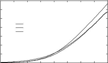
Let us explore a few implications of the capacity result (5.89) by comparing it with that for the AWGN channel. The capacity of the fading channel is always less than that of the AWGN channel with the same SNR. This follows directly from Jensen’s inequality, which says that if f is a strictly concave function and u is any random variable, then f u ≤ f u, with equality if and only if u is deterministic (Exercise B.2). Intuitively, the gain from

5 Note however that if the transmitter can really track the channel, one can do even better than this rate. We will see this next in Section 5.4.6.

203	5.4 Capacity of fading channels

the times when the channel strength is above the average cannot compensate for the loss from the times when the channel strength is below the average. This again follows from the law of diminishing marginal return on capacity from increasing the received power.

At low SNR, the capacity of the fading channel is

C = log 1 + h 2SNR ≈ h 2SNR log2 e = SNR log2 e ≈ Cawgn (5.92)

where Cawgn is the capacity of the AWGN channel and is measured in bits per symbol. Hence at low SNR the “Jensen’s loss” becomes negligible; this

is because the capacity is approximately linear in the received SNR in this regime. At high SNR,

C ≈ log h 2SNR = log SNR + log h 2 ≈ Cawgn + log h 2 (5.93)

i.e., a constant difference with the AWGN capacity at high SNR. This difference is −0 83 bits/s/Hz for the Rayleigh fading channel. Equivalently, 2.5 dB more power is needed in the fading case to achieve the same capacity as in the AWGN case. Figure 5.20 compares the capacity of the Rayleigh fading channel with the AWGN capacity as a function of the SNR. The difference is not that large for the entire plotted range of SNR.

5.4.6 Transmitter side information

Figure 5.20 Plot of AWGN capacity, fading channel capacity with receiver tracking the channel only (CSIR) and capacity with both transmitter and the receiver tracking the channel (full CSI). (A discussion of the latter is in Section 5.4.6.)

So far we have assumed that only the receiver can track the channel. But let us now consider the case when the transmitter can track the channel as well. There are several ways in which such channel information can be obtained at the transmitter. In a TDD (time-division duplex) system, the transmitter

7

6

5

Hz)/	4		Full CSI
			AWGN
/s			CSIR
(bitsC
	3
	2
	1
	0
	–20	–15	–10	–5	0	5	10	15	20
					SNR (dB)

204	Capacity of wireless channels

can exploit channel reciprocity and make channel measurements based on the signal received along the opposite link. In an FDD (frequency-division duplex) system, there is no reciprocity and the transmitter will have to rely on feedback information from the receiver. For example, power control in the CDMA system implicitly conveys some channel state information through the feedback in the uplink.

Slow fading: channel inversion

When we discussed the slow fading channel in Section 5.4.1, it was seen that with no channel knowledge at the transmitter, outage occurs whenever the channel cannot support the target data rate R. With transmitter knowledge, one option is now to control the transmit power such that the rate R can be delivered no matter what the fading state is. This is the channel inversion strategy: the received SNR is kept constant irrespective of the channel gain. (This strategy is reminiscent of the power control used in CDMA systems, discussed in Section 4.3.) With exact channel inversion, there is zero outage probability. The price to pay is that huge power has to be consumed to invert the channel when it is very bad. Moreover, many systems are also peak-power constrained and cannot invert the channel beyond a certain point. Systems like IS-95 use a combination of channel inversion and diversity to achieve a target rate with reasonable power consumption (Exercise 5.24).

Fast fading: waterfilling

In the slow fading scenario, we are interested in achieving a target data rate within a coherence time period of the channel. In the fast fading case, one is now concerned with the rate averaged over many coherence time periods. With transmitter channel knowledge, what is the capacity of the fast fading channel? Let us again consider the simple block fading model (cf. (5.86)):

y m = h m x m + w m

(5.94)

where h m = h remains constant over the th coherence period of Tc Tc 1 symbols and is i.i.d. across different coherence periods. The channel over L such coherence periods can be modeled as a parallel channel with L subchannels that fade independently. For a given realization of the channel gains h1 hL, the capacity (in bits/symbol) of this parallel channel is (cf. (5.39), (5.40) in Section 5.3.3)

									P h 2
max	1			L	log		1	+		(5.95)
P1 PL L =1									N0
subject to
		1 L
		L		=1 P = P						(5.96)

205 5.4 Capacity of fading channels

where P is the average power constraint. It was seen (cf. (5.43)) that the optimal power allocation is waterfilling:

=

1

N

+

P

−

0

(5.97)

h

2

where satisfies

1

L

1

N

+

−

2

= P

(5.98)

L =1

h 0

In the context of the frequency-selective channel, waterfilling is done over the OFDM sub-carriers; here, waterfilling is done over time. In both cases, the basic problem is that of power allocation over a parallel channel.

The optimal power P allocated to the th coherence period depends on the channel gain in that coherence period and , which in turn depends on all the other channel gains through the constraint (5.98). So it seems that implementing this scheme would require knowledge of the future channel states. Fortunately, as L → , this non-causality requirement goes away. By the law of large numbers, (5.98) converges to

						+	= P
	1			N
			−	0					(5.99)
				h 2

for almost all realizations of the fading process h m . Here, the expectation is taken with respect to the stationary distribution of the channel state. The parameter now converges to a constant, depending only on the channel statistics but not on the specific realization of the fading process. Hence, the optimal power at any time depends only on the channel gain h at that time:

P h =	1		−		N		0		+	(5.100)
						h	2

The capacity of the fast fading channel with transmitter channel knowledge is

C =	log 1 + P N0			2	bits/s/Hz	(5.101)
		h	h

Equations (5.101), (5.100) and (5.99) together allow us to compute the capacity.

We have derived the capacity assuming the block fading model. The generalization to any ergodic fading process can be done exactly as in the case with no transmitter channel knowledge.

206

Discussion

Figure 5.21 Pictorial representation of the waterfilling strategy.

Figure 5.22 Comparison of the fixed-rate and variable-rate schemes. In the fixed-rate scheme, there is only one code spanning many coherence periods. In the variable-rate scheme, different codes (distinguished by different shades) are used depending on the channel quality at that time. For example, the code in white is a low-rate code used only when the channel is weak.

Capacity of wireless channels

Figure 5.21 gives a pictorial view of the waterfilling power allocation strategy. In general, the transmitter allocates more power when the channel is good, taking advantage of the better channel condition, and less or even no power when the channel is poor. This is precisely the opposite of the channel inversion strategy. Note that only the magnitude of the channel gain is needed to implement the waterfilling scheme. In particular, phase information is not required (in contrast to transmit beamforming, for example).

The derivation of the waterfilling capacity suggests a natural variable-rate coding scheme (see Figure 5.22). This scheme consists of a set of codes of different rates, one for each channel state h. When the channel is in state h, the code for that state is used. This can be done since both the transmitter and the receiver can track the channel. A transmit power of P h is used when

	N0
	h[m] 2
1
λ	P[m] = 0
	P[m]
	Time m

2]m [h

Fixed-rate scheme

Variable-rate scheme

1		5							10				Time m

207	5.4 Capacity of fading channels

the channel gain is h. The rate of that code is therefore log 1+P h h 2/N0 bits/s/Hz. No coding across channel states is necessary. This is in contrast to the case without transmitter channel knowledge, where a single fixedrate code with the coded symbols spanning across different coherence time periods is needed (Figure 5.22). Thus, knowledge of the channel state at the transmitter not only allows dynamic power allocation but simplifies the code design problem as one can now use codes designed for the AWGN channel.

Waterfilling performance

Figure 5.20 compares the waterfilling capacity and the capacity with channel knowledge only at the receiver, under Rayleigh fading. Figure 5.23 focuses on the low SNR regime. In the literature the former is also called the capacity with full channel side information (CSI) and the latter is called the capacity with channel side information at the receiver (CSIR). Several observations can be made:

•At low SNR, the capacity with full CSI is significantly larger than the CSIR capacity.

•At high SNR, the difference between the two goes to zero.

•Over a wide range of SNR, the gain of waterfilling over the CSIR capacity is very small.

The first two observations are in fact generic to a wide class of fading models, and can be explained by the fact that the benefit of dynamic power allocation is a received power gain: by spending more power when the channel is good, the received power gets boosted up. At high SNR, however, the capacity is insensitive to the received power per degree of freedom and varying the amount of transmit power as a function of the channel state yields a minimal gain (Figure 5.24(a)). At low SNR, the capacity is quite sensitive to the received power (linear, in fact) and so the boost in received power from optimal transmit power allocation provides significant gain. Thus, dynamic

Figure 5.23 Plot of capacities with and without CSI at the transmitter, as a fraction of the AWGN capacity.

3
2.5
2					CSIR
C
					Full CSI
Cawgn
1.5
1
0.5
–20	–15	–10	–5	0	5	10

SNR (dB)