Fundamentals Of Wireless Communication

258	Multiuser capacity and opportunistic communication

sources of hindrance to implementing multiuser diversity in a real system. We will see a simple and practical scheme using an antenna array at the base-station that creates fast and large channel fluctuations even when the channel is originally slow fading with a small range of fluctuation.

6.7.1 Fair scheduling and multiuser diversity

As a case study, we describe a simple scheduling algorithm, called the proportional fair scheduler, designed to meet the challenges of delay and fairness constraints while harnessing multiuser diversity. This is the baseline scheduler for the downlink of IS-856, the third-generation data standard, introduced in Chapter 5. Recall that the downlink of IS-856 is TDMA-based, with users scheduled on time slots of length 1.67 ms based on the requested rates from the users (Figure 5.25). We have already discussed the rate adaptation mechanism in Chapter 5; here we will study the scheduling aspect.

Proportional fair scheduling: hitting the peaks

The scheduler decides which user to transmit information to at each time slot, based on the requested rates the base-station has previously received from the mobiles. The simplest scheduler transmits data to each user in a round-robin fashion, regardless of the channel conditions of the users. The scheduling algorithm used in IS-856 schedules in a channel-dependent manner to exploit multiuser diversity. It works as follows. It keeps track of the average throughput Tk m of each user in an exponentially weighted window of length tc. In time slot m, the base-station receives the “requested rates” Rk m , k = 1 K, from all the users and the scheduling algorithm simply transmits to the user k with the largest

Rk m

Tk m

among all active users in the system. The average throughputs Tk m are updated using an exponentially weighted low-pass filter:

T

m

+

1

=

1

−

1/tc Tk m + 1/tc Rk m

k = k

(6.56)

k

1

−

1/t

c

T

m

k

k

k

=

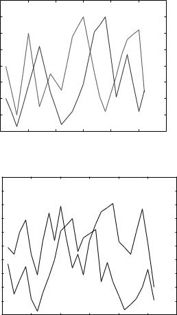
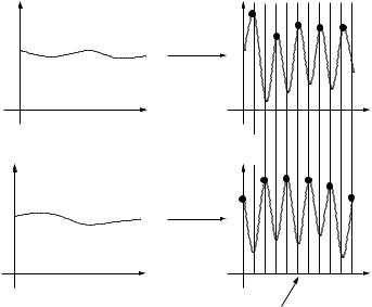
One can get an intuitive feel of how this algorithm works by inspecting Figures 6.14 and 6.15. We plot the sample paths of the requested data rates of two users as a function of time slots (each time slot is 1.67 ms in IS-856). In Figure 6.14, the two users have identical fading statistics. If the scheduling time-scale tc is much larger than the coherence time of the channels, then by symmetry the throughput of each user Tk m converges to the same quantity. The scheduling algorithm reduces to always picking the user with the highest

259	6.7 Multiuser diversity: system aspects

Figure 6.14 For symmetric channel statistics of users, the scheduling algorithm reduces to serving each user with the largest requested rate.

	1
	0.9
/Hz	0.8
bits/s
	0.7
in
rates	0.6
Requested	0.5
	0.4
	0.3
	0.2
	0	50	100	150	200	250	300
				Time slots

Figure 6.15 In general, with asymmetric user channel statistics, the scheduling algorithm serves each user when it is near its peak within the latency time-scale tc .

	1.2
	1.1
/s/Hz	1
	0.9
bits	0.8
in
rates	0.7
	0.6
Requested
	0.5
	0.4
	0.3
	0.2
	0	50	100	150	200	250	300
				Time slots

requested rate. Thus, each user is scheduled when its channel is good and at the same time the scheduling algorithm is perfectly fair in the long-term.

In Figure 6.15, due perhaps to different distances from the base-station, one user’s channel is much stronger than that of the other user on average, even though both channels fluctuate due to multipath fading. Always picking the user with the highest requested rate means giving all the system resources to the statistically stronger user, and would be highly unfair. In contrast, under the scheduling algorithm described above, users compete for resources not directly based on their requested rates but based on the rates normalized by their respective average throughputs. The user with the statistically stronger channel will have a higher average throughput.

Thus, the algorithm schedules a user when its instantaneous channel quality is high relative to its own average channel condition over the time-scale tc.

260	Multiuser capacity and opportunistic communication

In short, data are transmitted to a user when its channel is near its own peaks. Multiuser diversity benefit can still be extracted because channels of different users fluctuate independently so that if there is a sufficient number of users in the system, most likely there will be a user near its peak at any one time.

The parameter tc is tied to the latency time-scale of the application. Peaks are defined with respect to this time-scale. If the latency time-scale is large, then the throughput is averaged over a longer time-scale and the scheduler can afford to wait longer before scheduling a user when its channel hits a really high peak.

The main theoretical property of this algorithm is the following: With a very large tc (approaching ), the algorithm maximizes

K

log Tk

(6.57)

k=1

among all schedulers (see Exercise 6.28). Here, Tk is the long-term average throughput of user k.

Multiuser diversity and superposition coding

Proportional fair scheduling is an approach to deal with fairness among asymmetric users within the orthogonal multiple access constraint (TDMA in the case of IS-856). But we understand from Section 6.2.2 that for the AWGN channel, superposition coding in conjunction with SIC can yield significantly better performance than orthogonal multiple access in such asymmetric environments. One would expect similar gains in fading channels, and it is therefore natural to combine the benefits of superposition coding with multiuser diversity scheduling.

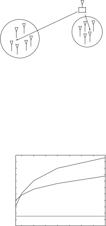
One approach is to divide the users in a cell into, say, two classes depending on whether they are near the base-station or near the cell edge, so that users in each class have statistically comparable channel strengths. Users whose current channel is instantaneously strongest in their own class are scheduled for simultaneous transmission via superposition coding (Figure 6.16). The user near the base-station can decode its own signal after stripping off the signal destined for the far-away user. By transmitting to the strongest user in each class, multiuser diversity benefits are captured. On the other hand, the nearby user has a very strong channel and the full degrees of freedom available (as opposed to only a fraction under orthogonal multiple access), and thus only needs to be allocated a small fraction of the power to enjoy very good rates. Allocating a small fraction of power to the nearby user has a salutary effect: the presence of this user will minimally affect the performance of the cell edge user. Hence, fairness can be maintained by a suitable allocation of power. The efficiency of this approach over proportional fair TDMA scheduling is quantified in Exercise 6.20. Exercise 6.19 shows that this strategy is in fact optimal in achieving any point on the boundary of

261	6.7 Multiuser diversity: system aspects

Figure 6.16 Superposition coding in conjunction with multiuser diversity scheduling. The strongest user from each cluster is scheduled and they are simultaneously transmitted to, via superposition coding.

the downlink fading channel capacity region (as opposed to the strategy of transmitting to the user with the best channel overall, which is only optimal for the sum rate and which is an unfair operating point in this asymmetric scenario).

Multiuser diversity gain in practice

We can use the proportional fair algorithm to get some more insights into the issues involved in realizing multiuser diversity benefits in practice. Consider the plot in Figure 6.17, showing the total simulated throughput of the 1 25 MHz IS-856 downlink under the proportional fair scheduling algorithm in three environments:

•Fixed Users are fixed, but there are movements of objects around them (2 Hz Rician, = Edirect/Especular = 5). Here Edirect is the energy in the direct

Figure 6.17 Multiuser diversity gain in fixed and mobile environments.

	1100
	1000
	900				Low mobility environment
s)	800
/
(kbits	700					Fixed environment
throughput	600
	500
	400
Total
	300	Latency time - scale		tc = 1.6 s
	200	Average SNR = 0 dB
	100				High mobility environment
	0
	2	4	6	8	10	12	14	16
			Number of users

262 Multiuser capacity and opportunistic communication

path that is not varying, while Especular refers to the energy in the specular or time-varying component that is assumed to be Rayleigh distributed.

The Doppler spectrum of this component follows Clarke’s model with a Doppler spread of 2 Hz.

• Low mobility Users move at walking speeds (3 km/hr, Rayleigh).

• High mobility Users move at 30 km/hr, Rayleigh.

The average channel gain h 2 is kept the same in all the three scenarios for fairness of comparison. The total throughput increases with the number of users in both the fixed and low mobility environments, but the increase is more dramatic in the low mobility case. While the channel varies in both cases, the dynamic range and the rate of the variations is larger in the mobile environment than in the fixed one (Figure 6.18). This means that over the latency time-scale (tc = 1 67 s in these examples) the peaks of the channel fluctuations are likely to be higher in the mobile environment, and the peaks are what determines the performance of the scheduling algorithm. Thus, the inherent multiuser diversity is more limited in the fixed environment.

Should one then expect an even higher throughput gain in the high mobility environment? In fact quite the opposite is true. The total throughput hardly increases with the number of users! It turns out that at this speed the receiver has trouble tracking and predicting the channel variations, so that the predicted channel is a low-pass smoothed version of the actual fading process. Thus, even though the actual channel fluctuates, opportunistic communication is impossible without knowing when the channel is actually good.

In the next section, we will discuss how the tracking of the channel can be improved in high mobility environments. In Section 6.7.3, we will discuss a scheme that boosts the inherent multiuser diversity in fixed environments.

6.7.2 Channel prediction and feedback

The prediction error is due to two effects: the error in measuring the channel from the pilot and the delay in feeding back the information to the base-station.

Figure 6.18 The channel varies much faster and has larger dynamic range in the mobile environment.

Channel

strength

Fixed environment

Dynamic

range

Time

Channel

strength

Mobile environment

Dynamic

range

Time

263 6.7 Multiuser diversity: system aspects

In the downlink, the pilot is shared between many users and is strong; so, the measurement error is quite small and the prediction error is mainly due to the feedback delay. In IS-856, this delay is about two time slots, i.e., 3 33 ms. At a vehicular speed of 30 km/h and carrier frequency of 1 9 GHz, the coherence time is approximately 2 5 ms; the channel coherence time is comparable to the delay and this makes prediction difficult.

One remedy to reduce the feedback delay is to shrink the size of the scheduling time slot. However, this increases the requested rate feedback frequency in the uplink and thus increases the system overhead. There are ways to reduce this feedback though. In the current system, every user feeds back the requested rates, but in fact only users whose channels are near their peaks have any chance of getting scheduled. Thus, an alternative is for each user to feed back the requested rate only when its current requested rate to average throughput ratio, Rk m /Tk m , exceeds a threshold . This threshold, , can be chosen to trade off the average aggregate amount of feedback the users send with the probability that none of the users sends any feedback in a given time slot (thus wasting the slot) (Exercise 6.22).

In IS-856, multiuser diversity scheduling is implemented in the downlink, but the same concept can be applied to the uplink. However, the issues of prediction error and feedback are different. In the uplink, the base-station would be measuring the channels of the users, and so a separate pilot would be needed for each user. The downlink has a single pilot and this amortization among the users is used to have a strong pilot. However, in the uplink, the fraction of power devoted to the pilot is typically small. Thus, it is expected that the measurement error will play a larger role in the uplink. Moreover, the pilot will have to be sent continuously even if the user is not currently scheduled, thus causing some interference to other users. On the other hand, the base-station only needs to broadcast which user is scheduled at that time slot, so the amount of feedback is much smaller than in the downlink (unless the selective feedback scheme is implemented).

The above discussion pertains to an FDD system. You are asked to discuss the analogous issues for a TDD system in Exercise 6.23.

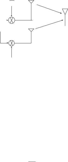
6.7.3 Opportunistic beamforming using dumb antennas

The amount of multiuser diversity depends on the rate and dynamic range of channel fluctuations. In environments where the channel fluctuations are small, a natural idea comes to mind: why not amplify the multiuser diversity gain by inducing faster and larger fluctuations? Focusing on the downlink, we describe a technique that does this using multiple transmit antennas at the base-station as illustrated in Figure 6.19.

Consider a system with nt transmit antennas at the base-station. Let hlk m be the complex channel gain from antenna l to user k in time m. In time m, the same symbol x m is transmitted from all of the antennas except that it is

264

Figure 6.19 Same signal is transmitted over the two antennas with time-varying phase and powers.

Multiuser capacity and opportunistic communication

√α (t)

h1k(t)

x(t)			h2k(t)	User k

√

e jθ(t)

1– α(t)

by a complex number

ej l m at antenna l, for l

=

1 n

,

m

multiplied

nt

lm = 1,

l

t

such that

l=1

preserving the total transmit power. The received

signal at

user k (see the basic downlink fading channel model in (6.50) for

comparison) is given by

ykm = lnt1

lm ej l m hlkm x m + wkm

(6.58)

=

In vector form, the scheme transmits qm x m at time m, where

ej 1 m

1m

qm

(6.59)

t

6

=

n m ej nt m

is a unit vector and

ykm = hkm qm x m + wkm

(6.60)

where hkm = h1km hnt km is the channel vector from the transmit antenna array to user k.

The overall channel gain seen by user k is now

hkm qm =	nt
	lm ej l m hlkm	(6.61)

l=1

The lm denote the fractions of power allocated to each of the transmit antennas, and the lm denote the phase shifts applied at each antenna to the

265

Figure 6.20 Pictorial representation of the slow fading channels of two users before (left) and after (right) applying opportunistic beamforming.

6.7 Multiuser diversity: system aspects

Before	After
opportunistic	opportunistic
beamforming	beamforming
Channel	Channel
strength	strength

User 1
t	t
Channel	Channel
strength	strength
User 2
t	t
	Transmission times

signal. By varying these quantities over time ( lm from 0 to 1 and lm from 0 to 2 ) , the antennas transmit signals in a time-varying direction, and fluctuations in the overall channel can be induced even if the physical channel gains hlkm have very little fluctuation (Figure 6.20).

As in the single transmit antenna system, each user k feeds back the overall received SNR of its own channel, hkm qm 2/N0, to the base-station (or equivalently the data rate that the channel can currently support) and the base-station schedules transmissions to users accordingly. There is no need to measure the individual channel gains hlkm (phase or magnitude); in fact, the existence of multiple transmit antennas is completely transparent to the users. Thus, only a single pilot signal is needed for channel measurement (as opposed to a pilot to measure each antenna gain). The pilot symbols are repeated at each transmit antenna, exactly like the data symbols.

The rate of variation of lm and lm in time (or, equivalently, of the transmit direction qm) is a design parameter of the system. We would like it to be as fast as possible to provide full channel fluctuations within the latency time-scale of interest. On the other hand, there is a practical limitation to how fast this can be. The variation should be slow enough and should happen at a time-scale that allows the channel to be reliably estimated by the users and the SNR fed back. Further, the variation should be slow enough

266	Multiuser capacity and opportunistic communication

to ensure that the channel seen by a user does not change abruptly and thus maintains stability of the channel tracking loop.

Slow fading: opportunistic beamforming

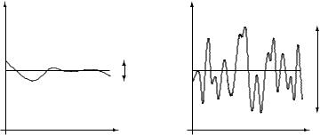
To get some insight into the performance of this scheme, consider the case of slow fading where the channel gain vector of each user k remains constant, i.e., hkm = hk, for all m. (In practice, this means for all m over the latency time-scale of interest.) The received SNR for this user would have remained constant if only one antenna were used. If all users in the system experience such slow fading, no multiuser diversity gain can be exploited. Under the proposed scheme, on the other hand, the overall channel gain hkm qm for each user k varies in time and provides opportunity for exploiting multiuser diversity.

Let us focus on a particular user k. Now if qm varies across all directions, the amplitude squared of the channel hkqm 2 seen by user k varies from 0 to hk 2. The peak value occurs when the transmission is aligned along the direction of the channel of user k, i.e., qm = hk/ hk (recall Example 5.2 in Section 5.3). The power and phase values are then in the beamforming configuration:

		l =	hlk 2		l	=	1 n
			hk 2
							t
	l = −arghlk					l = 1 nt

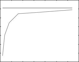
To be able to beamform to a particular user, the base-station needs to know individual channel amplitude and phase responses from all the antennas, which requires much more information to feedback than just the overall SNR. However, if there are many users in the system, the proportional fair algorithm will schedule transmission to a user only when its overall channel SNR is near its peak. Thus, it is plausible that in a slow fading environment, the technique can approach the performance of coherent beamforming but with only overall SNR feedback (Figure 6.21). In this context, the technique can be interpreted as opportunistic beamforming: by varying the phases and powers allocated to the transmit antennas, a beam is randomly swept and at any time transmission is scheduled to the user currently closest to the beam. With many users, there is likely to be a user very close to the beam at any time. This intuition has been formally justified (see Exercise 6.29).

Fast fading: increasing channel fluctuations

We see that opportunistic beamforming can significantly improve performance in slow fading environments by adding fast time-scale fluctuations on the overall channel quality. The rate of channel fluctuation is artificially sped up. Can opportunistic beamforming help if the underlying channel variations are already fast (fast compared to the latency time-scale)?

267	6.7 Multiuser diversity: system aspects

Figure 6.21 Plot of spectral efficiency under opportunistic beamforming as a function of the total number of users in the system. The scenario is for slow Rayleigh faded channels for the users and the channels are fixed in time. The spectral efficiency plotted is the performance averaged over the Rayleigh distribution. As the number of users grows, the performance approaches the performance of true beamforming.

	1.5
Hz	1.4				Coherent BF
/s/	1.3					Opp. BF
inbits
	1.2
throughput
	1.1
	1
Average
	0.9
	0.8
	0	5	10	15	20	25	30	35
				Number of users

The long-term throughput under fast fading depends only on the stationary distribution of the channel gains. The impact of opportunistic beamforming in the fast fading scenario then depends on how the stationary distributions of the overall channel gains can be modified by power and phase randomization. Intuitively, better multiuser diversity gain can be exploited if the dynamic range of the distribution of hk can be increased, so that the maximum SNRs can be larger. We consider two examples of common fading models.

•Independent Rayleigh fading In this model, appropriate for an environment where there is full scattering and the transmit antennas are spaced

sufficiently, the channel gains h1km hnt km are i.i.d. random

variables. In this case, the channel vector hkm is isotropically distributed, and hkm qm is circularly symmetric Gaussian for any choice of qm; moreover the overall gains are independent across the users. Hence, the

stationary statistics of the channel are identical to the original situation with one transmit antenna. Thus, in an independent fast Rayleigh fading environment, the opportunistic beamforming technique does not provide any performance gain.

•Independent Rician fading In contrast to the Rayleigh fading case, opportunistic beamforming has a significant impact in a Rician environment, particularly when the -factor is large. In this case, the scheme can significantly increase the dynamic range of the fluctuations. This is because the fluctuations in the underlying Rician fading process come from the diffused component, while with randomization of phase and powers, the fluctuations are from the coherent addition and cancellation of the direct path components in the signals from the different transmit antennas, in addition to the fluctuation of the diffused components. If the direct path