Fundamentals Of Wireless Communication

(b)

318	MIMO I: spatial multiplexing and channel modeling

7.3.6 Degrees of freedom and diversity

Degrees of freedom

Figure 7.15 Some examples of Ha. (a) Two clusters of scatterers, with all paths going through a single bounce.

(b) Paths scattered via multiple bounces.

Given the statistical model, one can quantify the spatial multiplexing capability of a MIMO channel. With probability 1, the rank of the random matrix Ha is given by

rank Ha = min number of non-zero rows, number of non-zero columns

(7.74)

(Exercise 7.6). This yields the number of degrees of freedom available in the MIMO channel.

The number of non-zero rows and columns depends in turn on two separate factors:

•The amount of scattering and reflection in the multipath environment. The more scatterers and reflectors there are, the larger the number of non-zero entries in the random matrix Ha, and the larger the number of degrees of freedom.

•The lengths Lt and Lr of the transmit and receive antenna arrays. With small antenna array lengths, many distinct multipaths may all be lumped into a

single resolvable path. Increasing the array apertures allows the resolution

(a)

		20				15
	|	15			|	10
	a kl				a kl
	|h	10			|h
		5				5
					30				30
		5			25	5			25
					20				20
		10				10
			15		15	15	20		15
	l – Transmitter bins		20	10	K – Receiver bins	l – Transmitter bins		10	K – Receiver bins
			25	5			25	5
				30				30

5°	10°	120°
Tx		Rx		–60°	5°	10°
40°						70°
–20° 10°				–120°
	15°		Tx
					10°
					15°	Rx
		–175°				–175°

319	7.3 Modeling of MIMO fading channels

of more paths, resulting in more non-zero entries of Ha and an increased number of degrees of freedom.

The number of degrees of freedom is explicitly calculated in terms of the multipath environment and the array lengths in a clustered response model in Example 7.1.

Example 7.1 Degrees of freedom in clustered response models

Clarke’s model

Let us start with Clarke’s model, which was considered in Example 2.2. In this model, the signal arrives at the receiver along a continuum set of paths, uniformly from all directions. With a receive antenna array of length Lr, the number of receive angular bins is 2Lr and all of these bins are non-empty. Hence all of the 2Lr rows of Ha are non-zero. If the scatterers and reflectors are closer to the receiver than to the transmitter (Figures 7.10(a) and 7.14(a)), then at the transmitter the angular spread %t (measured in terms of directional cosines) is less than the full span of 2. The number of non-empty rows in Ha is therefore Lt%t", such paths are resolved into bins of angular width 1/Lt. Hence, the number of degrees of freedom in the MIMO channel is

min Lt%t" 2Lr

(7.75)

If the scatterers and reflectors are located at all directions from the transmitter as well, then &t = 2 and the number of degrees of freedom in the MIMO channel is

min 2Lt 2Lr

(7.76)

the maximum possible given the antenna array lengths. Since the antenna separation is assumed to be half the carrier wavelength, this formula can also be expressed as

min nt nr

the rank of the channel matrix H

General clustered response model

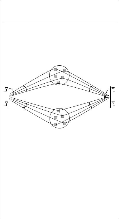
In a more general model, scatterers and reflectors are not located at all directions from the transmitter or the receiver but are grouped into several clusters (Figure 7.16). Each cluster bounces off a continuum of paths. Table 7.1 summarizes several sets of indoor channel measurements that support such a clustered response model. In an indoor environment, clustering can be the result of reflections from walls and ceilings, scattering from furniture, diffraction from doorway openings and transmission through soft partitions. It is a reasonable model when the size of the channel objects is comparable to the distances from the transmitter and from the receiver.

320	MIMO I: spatial multiplexing and channel modeling

Table 7.1 Examples of some indoor channel measurements. The Intel measurements span a very wide bandwidth and the number of clusters and angular spread measured are frequency dependent. This set of data is further elaborated in Figure 7.18.

	Frequency (GHz)	No. of clusters	Total angular spread (#)
USC UWB [27]	0–3	2–5	37
Intel UWB [91]	2–8	1–4	11–17
Spencer [112]	6.75–7.25	3–5	25.5
COST 259 [58]	24	3–5	18.5

Cluster of scatterers

φ t	Θ t,1	Θ r,1	φ r
	Θ t,2	Θ r,2
Transmit			Receive
array			array

Figure 7.16 The clustered response model for the multipath environment. Each cluster bounces off a continuum of paths.

In such a model, the directional cosines &r along which paths arrive are partitioned into several disjoint intervals: &r = k&rk. Similarly, on the transmit side, &t = k&tk. The number of degrees of freedom in the channel is

		Lr &tk"
min k	Lt &tk" k		(7.77)

For Lt and Lr large, the number of degrees of freedom is approximately

min Lt%t total Lr%r total			(7.78)
where
%t total = k	&tk and %r total = k	&rk	(7.79)

321	7.3 Modeling of MIMO fading channels

are the total angular spreads of the clusters at the transmitter and at the receiver, respectively. This formula shows explicitly the separate effects of the antenna array and of the multipath environment on the number of degrees of freedom. The larger the angular spreads the more degrees of freedom there are. For fixed angular spreads, increasing the antenna array lengths allows zooming into and resolving the paths from each cluster, thus increasing the available degrees of freedom (Figure 7.17).

One can draw an analogy between the formula (7.78) and the classic fact that signals with bandwidth W and duration T have approximately 2WT degrees of freedom (cf. Discussion 2.1). Here, the antenna array lengths Lt and Lr play the role of the bandwidth W , and the total angular spreads %t total and %r total play the role of the signal duration T.

Effect of carrier frequency

As an application of the formula (7.78), consider the question of how the available number of degrees of freedom in a MIMO channel depends on the carrier frequency used. Recall that the array lengths Lt and Lr are quantities normalized to the carrier wavelength. Hence, for a fixed physical length of the antenna arrays, the normalized lengths Lt and Lr increase with the carrier frequency. Viewed in isolation, this fact would suggest an increase in the number of degrees of freedom with the carrier frequency; this is consistent with the intuition that, at higher carrier frequencies, one can pack more antenna elements in a given amount of area on the device. On the other hand, the angular spread of the environment

Cluster of scatterers
1/L1	1/L1
Transmit	Receive
array	array
(a) Array length of L1
Cluster of scatterers
1/L2	1/L2
Transmit	Receive
array	array
(b) Array length of L2	> L1

Figure 7.17 Increasing the antenna array apertures increases path resolvability in the angular domain and the degrees of freedom.

322 MIMO I: spatial multiplexing and channel modeling

typically decreases with the carrier frequency. The reasons are two-fold:

•signals at higher frequency attenuate more after passing through or bouncing off channel objects, thus reducing the number of effective clusters;

•at higher frequency the wavelength is small relative to the feature size of typical channel objects, so scattering appears to be more specular in nature and results in smaller angular spread.

These factors combine to reduce %t total and %r total as the carrier frequency increases. Thus the impact of carrier frequency on the overall degrees of

freedom is not necessarily monotonic. A set of indoor measurements is shown in Figure 7.18. The number of degrees of freedom increases and then decreases with the carrier frequency, and there is in fact an optimal frequency at which the number of degrees of freedom is maximized. This example shows the importance of taking into account both the physical environment as well as the antenna arrays in determining the available degrees of freedom in a MIMO channel.

	0.45									7
	0.4						25
	0.35									6
							20		)
	0.3								−1	5
								1	(m
total	0.25						15	)	/λ	4
								(m
								-	c
Ω	0.2						1/λ		total	3
	0.15						10		Ω
										2
	0.1		Ω total in office
							5
	0.05		Ω total in townhouse							1		Office
	0 2		1/λ c				8 0			0 2		Townhouse
		3	4	5	6	7					3	4	5	6	7	8
			Frequency (GHz)									Frequency (GHz)
				(a)									(b)

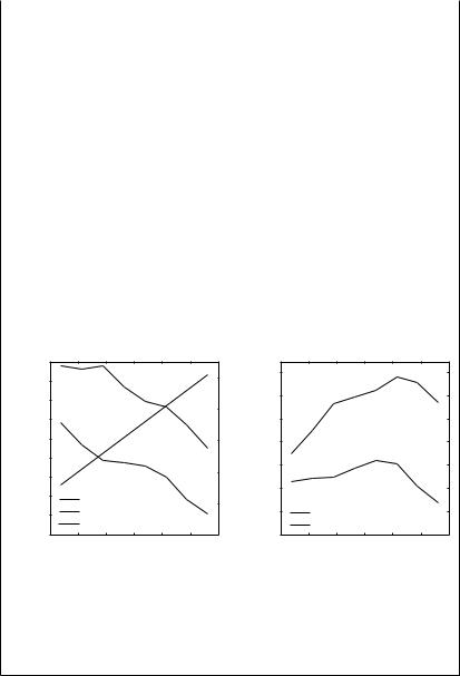
Figure 7.18 (a) The total angular spread total of the scattering environment (assumed equal at the transmitter side and at the receiver side) decreases with the carrier frequency; the normalized

array length increases proportional to 1/c . (b) The number of degrees of freedom of the MIMO channel, proportional to total/c , first increases and then decreases with the carrier frequency. The data are taken from [91].

Diversity

In this chapter, we have focused on the phenomenon of spatial multiplexing and the key parameter is the number of degrees of freedom. In a slow fading environment, another important parameter is the amount of diversity in the channel. This is the number of independent channel gains that have to be in a deep fade for the entire channel to be in deep fade. In the angular domain MIMO model, the amount of diversity is simply the number of non-zero

323

Figure 7.19 Angular domain representation of three MIMO channels. They all have four degrees of freedom but they have diversity 4, 8 and 16 respectively. They model channels with increasing amounts of bounces in the paths (cf. Figure 7.15).

7.3 Modeling of MIMO fading channels

r

r

r

n

n

n

nt

nt

nt

(a)

(b)

(c)

entries in Ha. Some examples are shown in Figure 7.19. Note that channels that have the same degrees of freedom can have very different amounts of diversity. The number of degrees of freedom depends primarily on the angular spreads of the scatters/reflectors at the transmitter and at the receiver, while the amount of diversity depends also on the degree of connectivity between the transmit and receive angles. In a channel with multiple-bounced paths, signals sent along one transmit angle can arrive at several receive angles (see Figure 7.15). Such a channel would have more diversity than one with single-bounced paths with signal sent along one transmit angle received at a unique angle, even though the angular spreads may be the same.

7.3.7 Dependency on antenna spacing

So far we have been primarily focusing on the case of critically spaced antennas (i.e., antenna separations t and r are half the carrier wavelength). What is the impact of changing the antenna separation on the channel statistics and the key channel parameters such as the number of degrees of freedom?

To answer this question, we fix the antenna array lengths Lt and Lr and vary the antenna separation, or equivalently the number of antenna elements. Let us just focus on the receiver side; the transmitter side is analogous. Given the antenna array length Lr, the beamforming patterns associated with the basis vectors er k/Lr k all have beam widths of 2/Lr (Figure 7.12). This dictates the maximum possible resolution of the antenna array: paths that arrive within an angular window of width 1/Lr cannot be resolved no matter how many antenna elements there are. There are 2Lr such angular windows, partitioning all the receive directions (Figure 7.20). Whether or not this maximum resolution can actually be achieved depends on the number of antenna elements.

Recall that the bins k can be interpreted as the set of all physical paths which have most of their energy along the basis vector et k/Lr . The bins dictate the resolvability of the antenna array. In the critically spaced caser = 1/2), the beamforming patterns of all the basis vectors have a single main lobe (together with its mirror image). There is a one-to-one correspondence between the angular windows and the resolvable bins k, and paths arriving in different windows can be resolved by the array (Figure 7.21). In

324	MIMO I: spatial multiplexing and channel modeling
Figure 7.20 An antenna array
				5			0		1
of length Lr partitions the
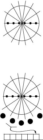
receive directions into 2Lr		4									2
angular windows. Here, Lr = 3
and there are six angular
windows. Note that because of
	3												3
symmetry across the 0 − 180
axis, each angular window
comes as a mirror image pair,
and each pair is only counted
as one angular window.		4									2
				5			0		1
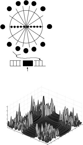
Figure 7.21 Antennas are
				L r = 3, nr = 6
critically spaced at half the
							0
wavelength. Each resolvable				5					1
bin corresponds to exactly one		4										2
angular window. Here, there
are six angular windows and
six bins.
	3												3

4					2
	5		0	1
0	1	2	3	4	5

k

Bins

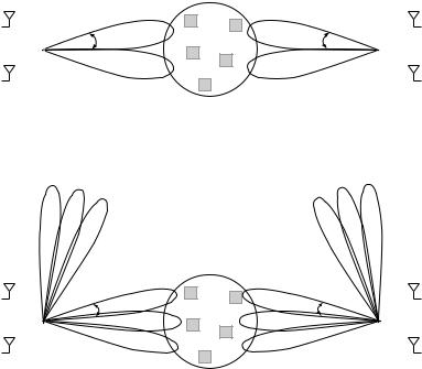
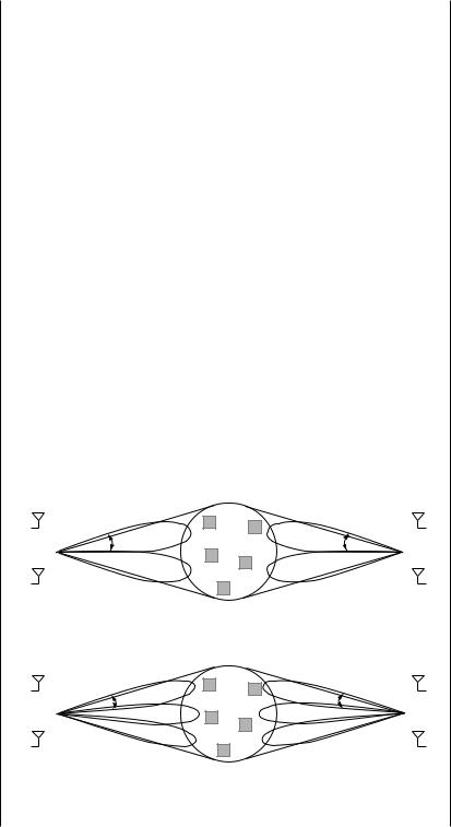
the sparsely spaced case ( r > 1/2), the beamforming patterns of some of the basis vectors have multiple main lobes. Thus, paths arriving in the different angular windows corresponding to these lobes are all lumped into one bin and cannot be resolved by the array (Figure 7.22). In the densely spaced case ( r < 1/2), the beamforming patterns of 2Lr of the basis vectors have a single main lobe; they can be used to resolve among the 2Lr angular windows. The beamforming patterns of the remaining nr − 2Lr basis vectors have no main lobe and do not correspond to any angular window. There is little received energy along these basis vectors and they do not participate significantly in the communication process. See Figure 7.23.

The key conclusion from the above analysis is that, given the antenna array lengths Lr and Lt, the maximum achievable angular resolution can be achieved by placing antenna elements half a wavelength apart. Placing antennas more sparsely reduces the resolution of the antenna array and can

325 7.3 Modeling of MIMO fading channels

						L r = 3, n r = 2
	L r = 3, n r = 5						0
						1		1
		0
	4		1			0		0
3					2
						1		1
2						3
3					2	0		0
						1
	4	0	1				0	1
0	1	2	3	4		0		1
						k		k
		Bins					Bins
		(a)					(b)

Figure 7.22 (a) Antennas are sparsely spaced. Some of the bins contain paths from multiple angular windows.

(b) The antennas are very sparsely spaced. All bins contain several angular windows of paths.

reduce the number of degrees of freedom and the diversity of the channel. Placing the antennas more densely adds spurious basis vectors which do not correspond to any physical directions, and does not add resolvability. In terms of the angular channel matrix Ha, this has the effect of adding zero rows and columns; in terms of the spatial channel matrix H, this has the effect of making the entries more correlated. In fact, the angular domain representation makes it apparent that one can reduce the densely spaced system to an equivalent 2Lt × 2Lr critically spaced system by just focusing on the basis vectors that do correspond to physical directions (Figure 7.24).

Increasing the antenna separation within a given array length Lr does not increase the number of degrees of freedom in the channel. What about increasing the antenna separation while keeping the number of antenna elements nr the same? This question makes sense if the system is hardware-limited rather than limited by the amount of space to put the antenna array in. Increasing the antenna separation this way reduces the beam width of the nr angular basis beamforming patterns but also increases the number of main lobes in each (Figure 7.25). If the scattering environment is rich enough such that the received signal arrives from all directions, the number of non-zero rows of the channel matrix Ha is already nr, the largest possible, and increasing the spacing does not increase the number of degrees of freedom in the channel. On the other hand, if the scattering is clustered to within certain directions, increasing the separation makes it possible for the scattered signal to be

326

Figure 7.23 Antennas are densely spaced. Some bins contain no physical paths.

Figure 7.24 A typical Ha when the antennas are densely spaced.

MIMO I: spatial multiplexing and channel modeling

L r = 3, n r = 10

9 0 1

8

2

7		3
8		2
9	0	1

0 1 2 3 4 5 6 7 8 9

k

Empty bins

L = 16, n = 50

	5
	4
|	3
a kl
|h	2
	1

50

			45
			40
10			35
20			30
			25
l – Transmitter bins 30		15	20
			K–Receiver bins
40		10
	50	5

received in more bins, thus increasing the number of degrees of freedom (Figure 7.25). In terms of the spatial channel matrix H, this has the effect of making the entries look more random and independent. At a base-station on a high tower with few local scatterers, the angular spread of the multipaths is small and therefore one has to put the antennas many wavelengths apart to decorrelate the channel gains.

Sampling interpretation

One can give a sampling interpretation to the above results. First, think of the discrete antenna array as a sampling of an underlying continuous array−Lr/2 Lr/2 . On this array, the received signal x s is a function of the

327

Figure 7.25 An example of a clustered response channel in which increasing the separation between a fixed number of antennas increases the number of degrees of freedom from 2 to 3.

7.3 Modeling of MIMO fading channels

		Cluster of scatterers
	1 / (nt∆1)	1 / (nr∆1)
Transmit			Receive
array	(a) Antenna separation of ∆1 = 1/2		array

	Cluster of scatterers
∆
1/(nt	)	1 / (nr∆2)
	2
Transmit		Receive
array		array

(b) Antenna separation of ∆2 > ∆1

continuous spatial location s −Lr/2 Lr/2 . Just like in the discrete case (cf. Section 7.3.3), the spatial-domain signal x s and its angular representation xa% form a Fourier transform pair. However, since only % −1 1 corresponds to directional cosines of actual physical directions, the angular representation xa% of the received signal is zero outside −1 1 . Hence, the spatial-domain signal x s is “bandlimited” to −W W, with “bandwidth” W = 1. By the sampling theorem, the signal x s can be uniquely specified by samples spaced at distance 1/2W = 1/2 apart, the Nyquist sampling rate. This is precise when Lr → and approximate when Lr is finite. Hence, placing the antenna elements at the critical separation is sufficient to describe the received signal; a continuum of antenna elements is not needed. Antenna spacing greater than 1/2 is not adequate: this is under-sampling and the loss of resolution mentioned above is analogous to the aliasing effect when one samples a bandlimited signal at below the Nyquist rate.

7.3.8 I.i.d. Rayleigh fading model

A very common MIMO fading model is the i.i.d. Rayleigh fading model: the entries of the channel gain matrix Hm are independent, identically