Chapter 12	HEAT TRANSFER ANALYSIS
	Post-processing Wall Heat Transfer Data in pro-STAR

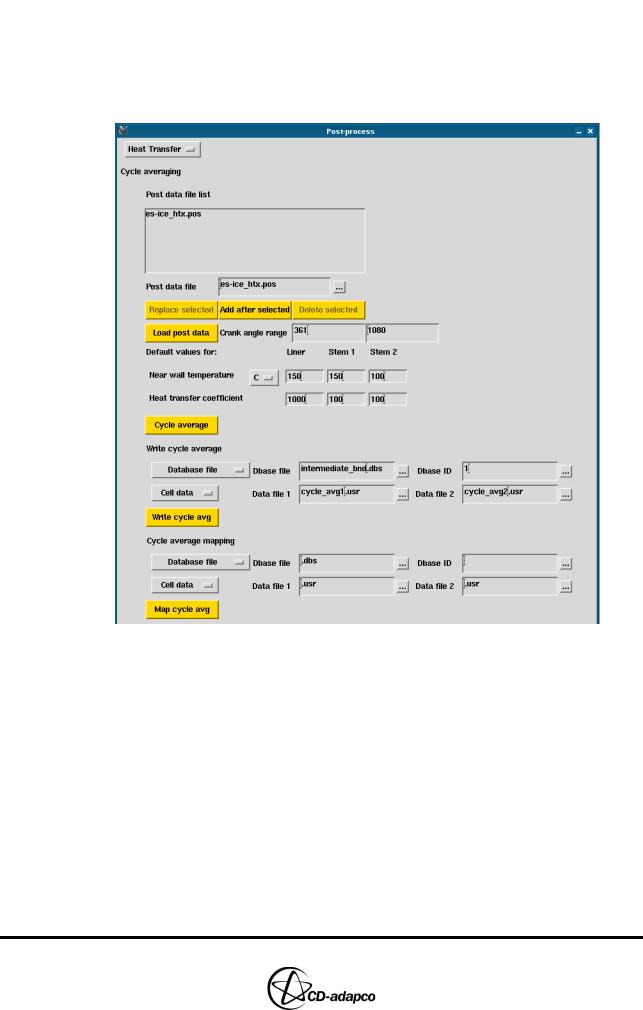
intermediate boundary grid on which the temperature values can be post-processed

•Set Data file 1 to cycle_avg1.usr and Data file 2 to cycle_avg2.usr to name the files that will contain the post-processing data

•Click the Write cycle avg button to create and store the cycle-averaged data

Figure 12-10 Post-process panel: Heat Transfer view

In your own cases, you can map the data onto a different surface mesh using the tools under the Cycle average mapping section.

•Close es-ice

Post-processing Wall Heat Transfer Data in pro-STAR

This section gives an example of post-processing cycle-averaged heat transfer data from es-ice in pro-STAR. In order to produce 3D contour plots of heat transfer, use the Get Post Data and Post Register Operations panels to import and manipulate data stored in the .usr files.

The plots to be created in this tutorial are Average Wall Boundary Temperature

(K), Average Heat Transfer Coefficient (W/m2-K) and Average Near-Wall Gas Temperature at Y-plus=100 (K).

Data file 1 (cycle_avg1.usr) contains six datasets summarised in Table

Version 4.20

12-9

HEAT TRANSFER ANALYSIS		Chapter 12
Post-processing Wall Heat Transfer Data in pro-STAR
12-1.
		Table 12-1: Datasets in Data file 1
	Register	Dataset
	Number
	Register 1	Average Heat Transfer Coefficient (W/m2-K)
	Register 2	Average Near-wall Gas Temperature (K)
	Register 3	Average Heat Flux (W/m2)
	Register 4	Average Wall Boundary Temperature (K)
	Register 5	Average Y-plus (Dimensionless)
	Register 6	Average Distance from Boundary to Y-plus=100 (m)

Data file 2 (cycle_avg2.usr) contains two datasets summarised in Table 12-2.

		Table 12-2: Datasets in Data file 2
	Register	Dataset
	Number
	Register 1	Average Heat Transfer Coefficient at Y-plus=100
		(W/m2-K)
	Register 2	Average Near-wall Gas Temperature at Y-plus=100 (K)

In this tutorial, you will use Register 4 and Register 1 from cycle_avg1.usr, and Register 2 from cycle_avg2.usr. Chapter 12, “After completing a simulation, you can use es-ice to generate a presentation that summarises the case features and analysis results. This presentation can be viewed using PowerPoint (Windows) or Open Office (Linux).” in the User Guide contains more information on this kind of dataset.

•Launch pro-STAR in the usual manner

•Enter the following commands to read the database file containing the cycle-averaged heat transfer data:

DBASE, OPEN, intermediate_bnd.dbs

DBASE, GET, 1

•Enter the following commands to view the surface mesh:

CSET, ALL

CPLOT

Plotting average wall boundary temperatures

To create a plot of Average Wall Boundary Temperature, import the relevant data from file cycle_avg1.usr using the Get Post Data panel.

12-10

Version 4.20

Chapter 12	HEAT TRANSFER ANALYSIS
	Post-processing Wall Heat Transfer Data in pro-STAR
•	From the menu bar, select Post >
	Get Post Data...
•	In the Get Post Data panel, use the
	file browser to select file

cycle_avg1.usr

•Select All (Register 1-6) from the

Registers drop-down menu

•Set the Data Format to Binary

•Accept the remaining default settings and click Apply, followed by Close

Next, adjust the colour scale to cover a range of 400 - 1100 K and select appropriate display options.

•Enter the following command to define the colour scale:

CSCALE, 14, USER, 400, 1100

•Enter the following commands to set up the display:

POPTION, CONTOUR VIEW, 1, -1, 1 AXIS, Z

ANGLE, 0 ZOOM, OFF

•Enter the following commands to create smooth contours by averaging the cell data values and then display the 3D temperature plot:

CAVERAGE, CSET

CPLOT

The resulting plot is shown in Figure 12-11.

Version 4.20

12-11

HEAT TRANSFER ANALYSIS	Chapter 12
Post-processing Wall Heat Transfer Data in pro-STAR

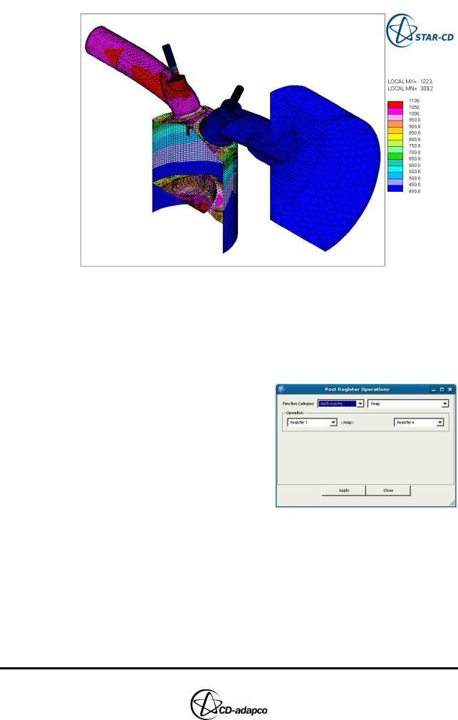
Figure 12-11 3D plot of cycle-averaged wall temperature (K)

Plotting average heat transfer coefficients

When plotting user data, pro-STAR always reads scalars from Register 4 (Registers 1, 2 and 3 are reserved for vector components X, Y and Z, respectively). In order to plot the cycle-averaged heat transfer coefficients, swap the data in Register 1 (heat transfer coefficients) for the data in Register 4 (wall boundary temperatures):

•From the menu bar, select Post >

Operate...

•In the Post Register Operations panel, set the Function Category to

Multi-register and select Swap from the second drop-down menu

•In the Operation box, select Register 1 from the first drop-down menu and Register 4 from the second drop-down menu

•Click Apply, then Close

•Enter the following commands to adjust the colour scale so that it covers a more suitable range and then plot the data using smooth contours:

CSCALE, 14, USER, 0, 1000

CPLOT

The resulting plot is shown in Figure 12-12.

12-12

Version 4.20