thin_section_microscopy

Guide to Thin Section Microscopy

Measuring lengths

2.2 Measurement of lengths

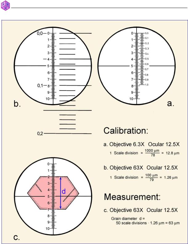
The measuring of distances is necessary for the determination of grain size, length-width ratios etc. For such measurements oculars are used that have a graticule (ocular micrometer) which must be calibrated. The graticule is commonly combined with the ocular crosshairs as a horizontally or vertically oriented scale attached to the E-W or N-S threads of the crosshairs, respectively (Fig. 2.2-1).

If objectives with increasing magnification are used, the image increases in size correspondingly. Therefore, the calibration of the graduations on the ocular scale must be carried out for each ocular-objective combination separately. The engraved magnification numbers on the objectives are only approximate values which would make a calibration based purely on calculations too imprecise.

For calibration, a specific scale is used, called an object micrometer, with a graduation of 10 µm per mark; 100 graduation marks add up to 1 mm. The object micrometer is put in a central stage position and, after focusing, is placed parallel and adjacent to the ocular scale (Fig. 2.2-1). In example (a) 100 graduation marks of the object micrometer, adding up to 1000 µm, correspond to 78 graduation marks on the ocular micrometer. At this magnification (objective 6.3x; ocular 12.5x) the distance between two graduation marks in the ocular is 1000 µm divided by 78. The interval is therefore 12.8 µm. Example (b) is valid for another combination (objective 63x; ocular 12.5x).

If, for example, a grain diameter needs to be determined, the number of graduation marks representing the grain diameter are counted and then multiplied by the calibration value for the particular objective-ocular combination (Fig. 2.2-1c).

The total error of the described procedure is a complex accumulated value. Both the object micrometer used for calibration and the ocular micrometer have a certain tolerance range. Errors occur with strongly magnifying lens systems because the image is not entirely planar, but has distortions in the peripheral domains. The largest error is commonly made by the human eye when comparing object and graduation. For increased accuracy it is important to use an objective with the highest possible magnification, such that the mineral grain covers a large part of the ocular scale.

Raith, Raase, Reinhardt – January 2011

25

Guide to Thin Section Microscopy

Measuring lengths

Raith, Raase, Reinhardt – January 2011

Figure 2.2-1: Calibration of the ocular micrometer and measurement of distances.

26

Raith, Raase, Reinhardt – January 2011

Guide to Thin Section Microscopy

Measuring thickness

2.3 Determination of thin section thickness

The birefringence of anisotropic minerals can be determined in approximation by comparing the interference colours to those of the Michel-Levy colour chart, or it can be done precisely using the compensation method. For both methods the thickness of the mineral in thin section must be known. Commonly, the thin section thickness is standardised to 25 resp. 30 µm. Abundant minerals such as quartz and feldspar would then show an interference colour of first-order grey to white. If these minerals are not present in the thin section, thickness is difficult to estimate for the inexperienced. In such a case, the thickness can be determined via the vertical travel of the microscope stage.

For focusing the image, microscopes are equipped with focusing knobs for coarse and fine adjustment. The instruction manuals supplied by the manufacturers contain information on the vertical travel per graduation mark. This value is 2 µm for many microscopes.

For measuring the thickness, an objective with high magnification and small depth of field (40x or 63x) is chosen and the surface of the cover slip is put into focus. This surface can be recognised by the presence of dust particles. The inexperienced user may put a fingerprint onto the surface! Now the fine adjustment is turned in the appropriate direction to decrease the distance between sample and objective. Eventually, the focus plane has passed the cover slip, and the interface between the embedding medium and the minerals appears. This is recognised by the surface roughness and the grinding marks on the thin section. Reducing the distance between sample and microscope stage further, the lower surface of the thin section with all its uneven features comes into focus. The path through the thin section can also be followed along cleavage planes and inclusions. Inexperienced users should repeat this procedure a couple of times and maybe make notes about, and cross-check, the positions of the various boundary surfaces using the scale at the focusing knobs.

For a precise determination of thickness using the upper and lower boundary surfaces of the thin section, it is necessary to turn the focal adjustment in one direction only, eliminating the mechanical backlash. If the thickness from the lower to the upper surface is measured, the starting position of the focal plane must be in the 1 mm thick glass slide. If moving in the reverse sense, the starting position must be in the 0.17 mm thick cover glass above the mineral surface.

The number of graduation marks by which the fine adjustment is turned in order to shift the focus from the lower to the upper boundary surface (or in the reverse direction) multiplied by the value given per graduation mark (e.g., 2 µm) results in a vertical travel distance h in µm. However, this distance is commonly not the true thickness of the section.

27

Guide to Thin Section Microscopy

Measuring thickness

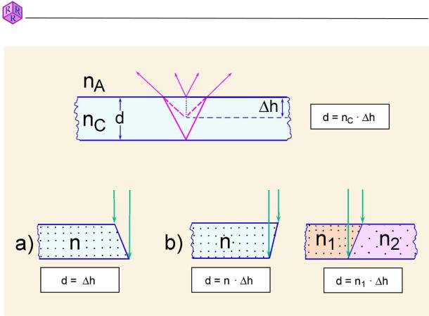
Due to light refraction against air, both boundary surfaces of the mineral in the thin section are not observed in their true position. The apparent position of the lower surface is influenced further by the refractive index of the mineral (Fig. 2.3-1, top).

The thickness is thus: d = ncrystal / nair * ǻh

whereby 'h, the vertical distance, is measured in number of graduation marks. The refraction index of the mineral should be known at least to the first decimal, which can be easily estimated.

For quartz, an example could be: d = 1.55/1.00 * 8.5

If one graduation mark corresponds to 2 µm, the result for the thin section thickness is:

d = 1.55/1.00 * 8.5 * 2 µm = 26.35 µm.

Calibration of travel

If the vertical travel is not known or maybe modified from extensive use of the microscope, it has to be calibrated. To this end, a cover glass is broken in two, and the thickness of the glass is determined near the broken edge with a micrometer tool. Such devices are available in every mechanical workshop. The cover glass fragment is then put onto a glass slide, with the fracture in the centre of view. Depending on the orientation of the fracture surface, there are two ways of calibration which should lead to the same result (Fig. 2.3-1a,b):

a)		d = h
b)	n = nglass § 1.5;	d = h * 1.5 (see above)

Raith, Raase, Reinhardt – January 2011

If the thickness of the cover glass measured with the micrometer tool was 168.4 µm, and the travel was 67.3, respectively 44.9, graduation marks, the calibration value per graduation mark would be

in case a) 168.4 µm / 67.3 = 2.5 µm;

in case b) 168.4 µm / 44.9 / 1.5 (nglass) = 2.5 µm.

The calibration error can have a number of sources. Mechanical tolerances of the micrometer and the microscope are normally small in comparison to observational errors in determining the different positions of the boundary surfaces. This error may be established from a series of measurements.

28

Guide to Thin Section Microscopy	Measuring thickness

Figure 2.3-1: Calibration of vertical travel and measurement of thickness.

Raith, Raase, Reinhardt – January 2011

29

Raith, Raase, Reinhardt – January 2011

Guide to Thin Section Microscopy

Crystal shape and symmetry

3. Morphological properties

3.1 Grain shape and symmetry

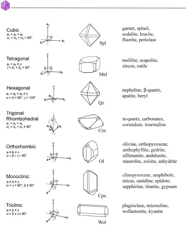
Natural minerals as well as synthetic substances show a considerable variety of crystal forms. The symmetry of the "outer" crystal form of a specific mineral species is an expression of the symmetry of the "inner" atomic structure. According to their symmetry characteristics all known crystalline phases can be assigned to one of the seven groups of symmetry (= crystal systems) (Fig. 3.1-1).

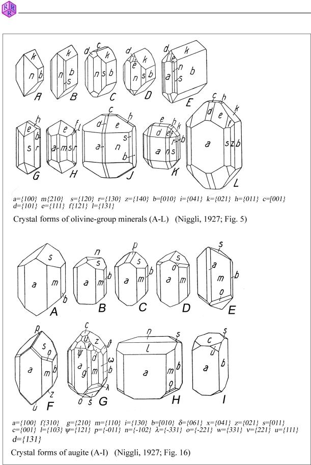
Combination of crystal faces: Depending on growth conditions, a mineral species can occur in different crystal forms through combinations of different crystal faces. Fig. 3.1-2 shows examples of the variety of crystal forms of olivine and augite from natural occurrences.

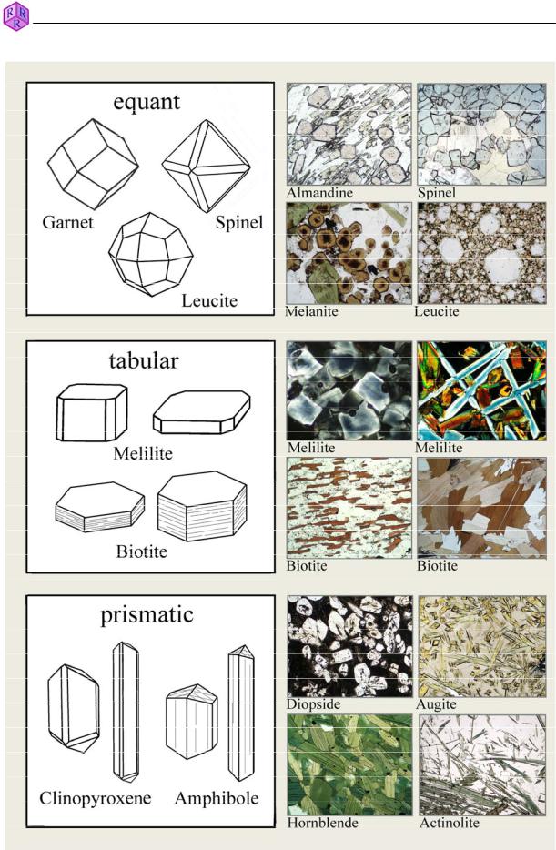
Habit: Crystals may also have different proportions, even if they have the same crystal faces developed. That means they differ in the relative size of crystal faces to each other. Figure 3.1-3 shows crystals of different habit using the examples spinel, garnet, sodalite and leucite (all equant), melilite, mica (flaky, platy to short-columnar) and clinopyroxene and amphibole (acicular, prismatic).

Crystal shape: Euhedral crystals, which are crystals completely bound by rational crystal faces reflect unobstructed growth (such as crystallisation in a melt, Fig. 3.1-4, or in amygdales, caverns, pores etc.), or they form if a particular mineral has the tendency to impose its crystal shape and faces onto the adjacent, "weaker" ones (crystalloblastic series; Fig. 3.1-4).

Subhedral and anhedral grain shapes are observed if the mineral’s characteristic shape could only develop partly, or not at all, if thermally induced annealing creates polycrystalline grain aggregates (Fig. 3.1-6), or if dissolution or melting processes lead to a "rounding" of crystal edges.

Fast crystallization from a melt can produce skeletal crystals or hollow shapes (Fig. 3.1-7). Minute feathery, dendritic or acicular crystals grow in undercooled melt (glass) (Fig. 3.1-8).

In the two-dimensional thin section image, the 3-D crystal shape of a mineral species has to be deduced from the outlines of the different crystal cross-sections (Fig. 3.1-9). For the rockforming minerals, the schematic crystal drawings in the tables of Tröger et al. (1979) may be used as a reference. Fig. 3.1-10 shows the correlation between crystal shape and crystal sections for a member of the clinopyroxene group.

30

Raith, Raase, Reinhardt – January 2011

Guide to Thin Section Microscopy	Crystal shape and symmetry

Figure 3.1-1: Crystal systems

31

Guide to Thin Section Microscopy

Crystal shape and symmetry

Raith, Raase, Reinhardt – January 2011

Figure 3.1-2: Variety of crystal forms shown by single mineral species through combinations of different crystal faces, as seen in augite and olivine.

32

Raith, Raase, Reinhardt – January 2011

Guide to Thin Section Microscopy	Crystal shape and symmetry

Figure 3.1-3: Habit of crystals

33

Guide to Thin Section Microscopy

Crystal shape and symmetry

Raith, Raase, Reinhardt – January 2011

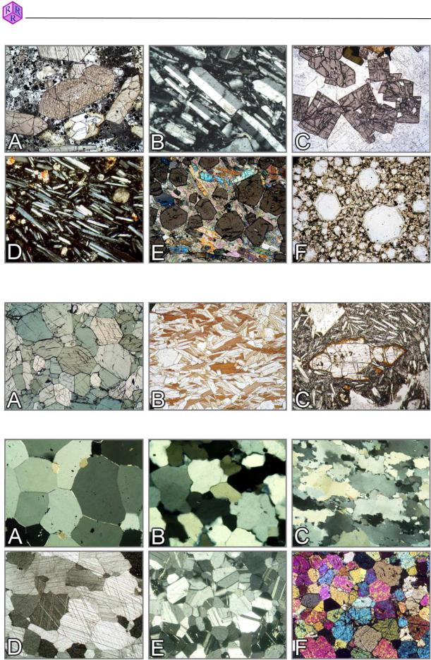
Figure 3.1-4: Euhedral grain shape

A: Augite (basalt), B: Sanidine (trachyte); C: Zircon (syenite pegmatite); D: Plagioclase (basalt); E: Garnet (garnet-kyanite micaschist); F: Leucite (foidite).

Figure 3.1-5: Subhedral grain shape

A: Amphibolite; B: Biotite-muscovite schist; C: Olivine in basalt

Figure 3.1-6: Anhedral grain shape

Granoblastic textures of quartzite (A to C), marble (D), anorthosite (E) and fayalite fels (F).

34