42  introduction to statistics for biomedical engineers

Some examples or questions asked by biomedical engineers that require comparing two population means include the following:

1.Is one chemotherapy drug more effective than a second chemotherapy drug in reducing the size of a cancerous tumor?

2.Is there a difference in postural stability between young and elderly populations?

3.Is there a difference in bone density for women who are premenopausal versus those who are postmenopausal?

4.Is titanium a stronger material for bone implants than steel?

5.For MRI, does one type of pulse sequence perform better than another in detecting white matter tracts in the brain?

6.Do drug-eluting intravascular stents prevent restenosis more effectively than noncoated stents?

In answering these type of questions, biomedical engineers often collect samples from two different groups of subjects or from one group of subjects but under two different conditions. For a specific measure that represents the samples, a sample mean is typically estimated for each group or under each of two conditions. Comparing the means from two populations reflected in two sets of data is probably the most reported statistical analysis in the scientific and engineering literature and may be accomplished using something known as a t test.

5.1.1 The t Test

When performing the t test, we are asking the question, “Are the means of two populations really different?” or “Would we see the observed differences simply because of random chance?” The two populations are reflected in data that have been collected under two different conditions. These conditions may include two different treatments or processes.

To address this question, we use one of the following two tests, depending on whether the two data sets are independent or dependent on one another:

1.Unpaired t test for two sets of independent data

2.Paired t test for two sets of dependent data

Before we describe each type of t test, we need to discuss the notion of hypothesis testing.

5.1.1.1 Hypothesis Testing

Whenever we perform statistical analysis, we are testing some hypothesis. In fact, before we even collect our data, we formulate a hypothesis and then carefully design our experiment and collect

Statistical Inference  43

and analyze the data to test the hypothesis. The outcome of the statistical test will allow us, if the assumed probability model is valid, to accept or reject the hypothesis and do so with some level of confidence.

There are basically two forms of hypotheses that we test when performing statistical analysis. There is the null hypothesis and the alternative hypothesis.

The null hypothesis, denoted as H0, is expressed as follows for the t test comparing two population means, 1 and 2:

H0: 1 = 2.

The alternative hypothesis, denoted as H1, is expressed as one of the following for the t test comparing two population means, 1 and 2:

H1: 1	≠ 2	(two-tailed t test),
H1: 1	< 2	(one tailed t test),
or
H1: 1	> 2	(one-tailed t test).

If the H1 is of the first form, where we do not know in advance of the data collection which mean will be greater than the other, we will perform a two-tailed test, which simply means that the level of significance for which we accept or reject the null hypothesis will be double that of the case in which we predict in advance of the experiment that one mean will be lower than the second based on the physiology or the engineering process or other conditions affecting experimental outcome. Another way to express this is that with a one-tailed test, we will have greater confidence in rejecting or accepting the null hypothesis than with the two-tailed condition.

5.1.1.2 Applying the t Test

Now that we have stated our hypotheses, we are prepared to perform the t test. Given two populations with n1 and n2 samples, we may compare the two population means using a t test. It is important to remember the underlying assumptions made in using the t test to compare two population means:

1.The underlying distributions for both populations are normal.

2.The variances of the two populations are approximately equal: s12 = s22.

These are big assumptions we make when n1 and n2 are small. If these assumptions are poor for the data being analyzed, we need to find different statistics to compare the two populations.

44  introduction to statistics for biomedical engineers

Given two sets of sampled data, xi and yi, the means for the two populations or processes reflected in the sampled data can be compared using the following t statistic:

5.1.1.3 Unpaired t Test

The unpaired t statistic may be estimated using:

T =	x − y
	(n1 − 1)Sx 2 + (n2 − 1)Sy 2
	n1 + n2 − 2



,

1 + 1 n1 n2

where n	1	is the number of x		i	observations, n		2	is the number of y	i	observations, S 2 is the sample
					–					x
variance of xi ,		2				is the sample average for xi , and y is the sample average
	Sy		= sample variance of yi, x

for yi .

Once the T statistic has been computed, we can compare our estimated T value to t values given in a table for the t distribution. More specifically, if we want to reject the null hypothesis with 1 − α level of confidence, then we need to determine whether our estimated T value is greater than the t value entry in the t table associated with a significance level of α (one-sided t test) or α/2 (twosided t test). In other words, we need to know the t value from the t distribution for which the area under the t curve to the right of t is α. Our estimated T must be greater than this t to reject the null hypothesis with 1 − α level of confidence.

Thus, we compare our T value to the t distribution table entry for

t(α, n1 + n2 − 2)	(one-sided)
or
t(α/2, n1 + n2 − 2)	(two-sided),

where α is the level of significance (equal to 1 – level of confidence), and n1 and n2 are the number of samples from each of the two populations being compared.

Note that α is the level of significance at which we want to accept or reject our hypothesis. For most research, we reject the null hypothesis when α ≤ 0.05. This corresponds to a confidence level of 95%.

For example, if we want to reject our null hypothesis with a confidence level of 95%, then for a one-sided t test, our estimated T must be greater than t (0.05, n1 + n2 – 2) to reject H0 and accept H1 with 95% confidence or a significance level of 0.05 or less. Remember that our confidence = (1– 0.05) × 100%. This test was for H1: µ1 < µ2 or µ1 > µ2 (one-sided). If our H1 was H1:

Statistical Inference  45

µ1 ≠ µ2, then our measured T must be greater than t (0.05/2, n1 + n2 – 2) to reject the null hypothesis with the same 95% confidence.

Thus, to test the following alternative hypotheses:

1.For H1: µ1 ≠ µ2: Use two-tail t test. For (α < 0.05), the estimated T > t (0.025, n1 + n2 − 2) to reject H0 with 95% confidence.

2.For H1: µ1 < µ2 or H1: µ1 < µ2: Use one-tail t test. For (α < 0.05), estimated T > t (0.05, n1 + n2 − 2) to reject H0 with 95% confidence.

αis also referred to as the type I error. For the t test, α is the probability of observing a measured T value greater than the table entry, t (α; df  ) if the true means of two underlying populations, x and y, were actually equal. In other words, there is no significant (α < 0.05) difference in the two population means, but the sampled data analysis led us to conclude that there is a difference and thus reject the null hypothesis. This is referred to as a type I error.

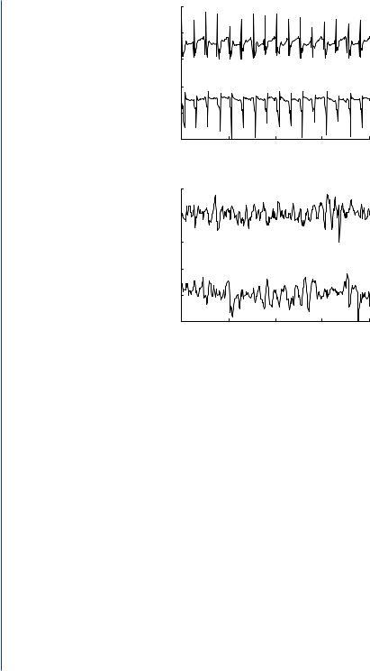
Example 5.1 An example of a biomedical engineering challenge where we might use the t test to improve the function of medical devices is in the development of implantable defibrillators for the detection and treatment of abnormal heart rhythms [13]. Implantable defibrillators are small electronic devices that are placed in the chest and have thin wires that are placed in the chambers of the heart. These wires have electrodes that detect the small electrical current traversing the heart muscle. Under normal conditions, these currents follow a very orderly pattern of conduction through the heart muscle. An example of an electrogram, or record of electrical activity that is sensed by an electrode, under normal conditions is given in Figure 5.1. When the heart does not function normally and enters a state of fibrillation (Figure 5.1), whereby the heart no longer contracts normally or pumps blood to the rest of the body, the device should shock the heart with a large electrical current from the device in an attempt to convert the heart rhythm back to normal. For a number of reasons, it is important that the device accurately detect the onset of life-threatening arrhythmias, such as fibrillation, and administer an appropriate shock. To administer a shock, the device must use some sort of signal processing algorithms to automatically determine that the electrogram is abnormal and characteristic of fibrillation.

One algorithm that is used in most devices for differentiating normal heart rhythms from fibrillation is a rate algorithm. This algorithm is basically an amplitude threshold crossing algorithm whereby the device determines how often the electrogram exceeds an amplitude threshold in a specified period of time and then estimates a rate from the detected threshold crossings. Figure 5.2 illustrates how this algorithm works.

Before such an algorithm was put into implantable defibrillators, researchers and developers had to demonstrate whether the rate estimated by such a device truly differed between normal and

46  introduction to statistics for biomedical engineers

	1
	0.5
amplitude	0					AFLUT
	1
	0.5
	0	0	1	2	3	4

time (s)

	1
	0.5
amplitude	0					AF
	1
	0.5
	0	0	1	2	3	4

time (s)

FIGURE 5.1: Electrogram recordings measured from electrodes placed inside the left atrium of the heart. For each rhythm, there are two electrogram recordings taken from two different locations in the atrium: atrial flutter (AFLUT) and atrial fibrillation (AF).

fibrillatory rhythms. It was important to have little overlap between the normal and fibrillatory rhythms so that a rate threshold could be established, whereby rates that exceeded the threshold would lead to the device administering a shock. For this algorithm to work, there must be a significant difference in rates between normal and fibrillatory rhythms and little overlap that would lead to shocks being administered inappropriately and causing great pain or risk the induction of fibrillation. Overlap in rates between normal and fibrillatory rhythms could also result in the device missing detection of fibrillation because of low rates.

To determine if rate is a good algorithm for detecting fibrillatory rhythms, investigators might actually record electrogram signals from actual patients who have demonstrated normal or fibrillatory rhythms and use the rate algorithm to estimate a rate and then compare the mean rates for normal rhythms against mean rates for fibrillatory rhythms. For example, let us assume

Statistical Inference  47

FIGURE 5.2: A heart rate is estimated from an electrogram using an amplitude threshold algorithm. Whenever the amplitude of the electrogram signal (solid waveform) exceeds an amplitude threshold (solid gray horizontal line) within a specific time interval (shaded vertical bars), an “event” is detected. A rate is calculated by counting the number of events in a certain time period.

investigators collected 15-second electrogram recordings for examples of fibrillatory (n1 = 10) and nonfibrillatory rhythms (n2 = 11) in 21 patients. We note that the fibrillatory data were collected from different subjects than the normal data. Thus, we do not have blocking in this experimental design.

A rate was estimated, using the device algorithm, for each individual 15-second recording. Figure 5.3 shows a box-and-whisker plot for each of the two data sets.

The descriptive statistics for the two data sets are given by the following table:

	Nonfibrillatory	Fibrillatory
	electrograms	electrograms
	(n1 = 11)	(n2 = 10)
Mean	96.82	239.0
Standard deviation	22.25	55.3

There are several things to note from the plots and descriptive statistics. First, the sample size is small; thus, it is likely that the variability of electrogram recordings from normal and fibrillatory rhythms is not adequately represented. Moreover, the data are skewed and do not appear to be well modeled by a normal distribution. Finally, the variability in rates appears to be much greater for fibrillatory rhythms than for normal rhythms. Thus, some of the assumptions we make regarding

48  introduction to statistics for biomedical engineers

Estimated Rate

Rate (BPM)	300
	200
Estimated
	100
	nonf ibrillatory	f ibrillatory

Rhythm Type

FIGURE 5.3: Box-and-whisker plot for rate data estimated from samples of nonfibrillatory and fibrillatory heart rhythms.

the normality of the populations and the equality of variances are probably violated in applying the t test. However for the purpose of illustration, we will perform a t test using the unpaired t statistic.

To find an estimated T statistic from our sample data, we plug in the means, variances, and sample sizes into the equation for the unpaired T statistic. We turn the crank and find that for this example, the estimated t value is 7.59. If we look at our t tables for [11 + 10 − 2] degrees of freedom, we can reject H0 at α < 0.005 because our estimated T value exceeds the t table entries for α = 0.05 (t = 1.729), α = 0.01 (t = 2.539), and α = 0.005 (t = 2.861).

Thus, we reject the null hypothesis with (1 − 0.005) × 100% confidence and state that mean heart rate for fibrillatory rhythms is greater than mean heart rate for normal rhythms. Thus, the rate algorithm should perform fairly well in differentiating normal from fibrillatory rhythms. However, we have only tested the population means. As one may see in Figure 5.3, there is some overlap in individual samples between normal and fibrillatory rhythms. Thus, we might expect the device to make errors in administering shock inappropriately when the heart is in normal but accelerated rhythms (as in exercise), or the device may fail to shock when the heart is fibrillating but at a slow rate or with low amplitude.

In applying the t test, it is important to note that you can never prove that two means are equal. The statistics can only show that a specific test cannot find a difference in the population means, and, not finding a difference is not the same as proving equality. The null or default hypothesis is that there is no difference in the means, regardless of what the true difference is between the two means. Not finding a difference with the collected data and appropriate statistical test does not

Statistical Inference  49

mean that the means are proved equal. Thus, we do not accept the null hypothesis with a level of significance. We simply accept the null hypothesis and do not accept with a confidence or significance level. We only assign a level of confidence when we reject the null hypothesis.

5.1.1.4 Paired t Test

In the previous example, we used an unpaired t test because the two data sets came from two different, unrelated, groups of patients. The problem with such an experimental design is that differences in the two patient populations may lead to differences in mean heart rate that have nothing to do with the actual heart rhythm but rather differences in the size or age of the hearts between the two groups of patients or some other difference between patient groups. A better way to conduct the previous study is to collect our normal and fibrillatory heart data from one group of patients. A single defibrillator will only need to differentiate normal and fibrillatory rhythms within a single patient. By blocking on subjects we can eliminate the intersubject variability in electrogram characteristics that may plague the rate algorithm from separating populations. It may be more reasonable to assume that rates for normal and fibrillatory rhythms differ more within a patient than across patients. In other words, for each patient, we collect an electrogram during normal heart function and fibrillation. In such experimental design, we would compare the means of the two data sets using a paired t test.

We use the paired t test when there is a natural pairing between each observation in data set, X, with each observation in data set, Y. For example, we might have the following scenarios that warrant a paired t test:

1.Collect blood pressure measurements from 8 patients before and after exercise.

2.Collect both MR and CT data from the same 20 patients to compare quality of blood vessel images.

3.Collect computing time for an image processing algorithm before and after a change is made in the software.

In such cases, the X and Y data sets are no longer independent. In the first example above, because we are collecting the before and after data from the same experimental units, the physiology and biological environment that impacts blood pressure before exercise in each patients also affects blood pressure after exercise. Thus, there are a number of variables that impact blood pressure that we cannot directly control but whose effects on blood pressure (beside the exercise effect) can be controlled by using the same experimental units (human subjects in this case) for each data set. In such cases, the experimental units serve as their own control. This is typically the preferred experimental design for comparing means.

50  introduction to statistics for biomedical engineers

For the paired t test, we again have a null hypothesis and an alternative hypothesis as stated above for the unpaired t test. However, in a paired t test, we use a t test on the difference, Wi = Xi − Yi, between the paired data points from each of the two populations.

We now calculate the paired T statistic: (n = number of pairs)

T =		W				,
	Sw /
				n

—

where W is the average difference of the differences, Wi, and Sw is the standard deviation of the differences, Wi.

As for the unpaired t test, we now have an estimated T value that we can compare with the t values in the table for the t distribution to determine if the estimated T value lies in the extreme values (greater than 95%) of the t distribution.

To reject the null hypothesis at a significance level of α (confidence level of 1 – α), our estimated T value must be greater than t (α, n − 1), where n is the number of pairs of data.

If the estimated T value exceeds t (α, n − 1), we reject H0 and accept H1 at a significance level of α or a confidence level of 1 − α.

Once again, if H1: µ1 < µ2 or H1: µ1 < µ2, we perform a one-sided test where our T statistic must be greater than t (α, n − 1) to reject the null hypothesis at a level of α. If the null hypothesis that we begin with before the experiment is H1: (µ1 ≠ µ2), then we perform a two-sided test, and the T statistic must be greater than t (α/2, n − 1) to reject the null hypothesis at a significance level of α.

5.1.1.5 Example of a Biomedical Engineering Challenge

In relation to abnormal heart rhythms discussed previously, antiarrhythmic drugs may be used to slow or terminate an abnormal rhythm, such as fibrillation. For example, a drug such as procainamide may be used to terminate atrial fibrillation. The exact mechanism whereby the drug leads to termination of the rhythm is not exactly known, but it is thought that the drug changes the refractory period and conduction velocity of the heart cells [8]. Biomedical engineers often use signal processing on the electrical signals generated by the heart as an indirect means for studying the underlying physiology. More specifically, engineers may use spectral analysis or Fourier analysis to look at changes in the spectral content of the electrical signal, such as the electrogram, over time. Such changes may tell us something about the underlying electrophysiology.

For example, spectral analysis has been used to look at changes in the frequency spectrum of atrial fibrillation with drug administration. In one such study [8], biomedical engineers were interested in looking at changes in median frequency of atrial electrograms after drug administration. Figure 5.4 shows an example of the frequency spectrum for atrial fibrillation and the location

							Statistical Inference		51
	1.2
	1			peak power
power	0.8
				median frequency (4–9 Hz)
normalized	0.6
	0.4
	0.2
	0	0	5	10	15	20	25	30

frequency (Hz)

FIGURE 5.4: Frequency spectrum for an example of atrial fibrillation. Median frequency is defined as that frequency that divides the area under the power curve in the 4- to 9-Hz band in half.

of the median frequency, which is the frequency that divides the power of the spectrum (area under the spectral curve between 4 and 9 Hz) in half. One question posed by the investigators is whether median frequency decreases after administration of a drug such procainamide, which is thought to slow the electrical activity of the heart cells.

Thus, an experiment was conducted to determine whether there was a significant difference in mean median frequency between fibrillation before drug administration and fibrillation after drug administration. Electrograms were collected in the right atrium in 11 patients before and after the drug was administered. Fifteen-second recordings were evaluated for the frequency spectrum, and the median frequency in the 4- to 9-Hz frequency band was estimated before and after drug administration.

Figure 5.5 illustrates the summary statistics for median frequency before and after drug administration. The question is whether there was a significant decrease in median frequency after

52  introduction to statistics for biomedical engineers

Median Frequency

	7
MF	6
Estimated	5
	4
	3
	Before Drug	After Drug

FIGURE 5.5: Box-and-whisker plot for median frequency estimated from samples of atrial fibrillation recorded before, and after a drug was administered.

administration of procainamide. In this case, the null hypothesis is that there is no change in mean median frequency after drug administration. The alternative hypothesis is that mean median frequency decreases after drug administration. Thus, we are comparing two means, and the two data sets have been collected from one set of patients. We will require a paired t test to reject or accept the null hypothesis.

Before drug	After drug	Wi
4.30	2.90	1.4
4.15	2.97	1.18
3.80	3.20	0.60
5.10	3.30	1.80
4.30	3.75	0.55
7.20	5.35	1.85
6.40	5.10	1.30
6.20	4.90	1.30
6.10	4.80	1.30
5.00	3.70	1.30
5.80	4.50	1.30

Statistical Inference  53

To perform a paired t test, we create another column, Wi, as noted in the table above. We

— —

find the following for Wi: W = 1.262 and Sw = 0.402. If we use these estimates for W and Sw in our equation for the paired T statistic, we find that T = 10.42 for n = 11 pairs of data. If we compare our estimated T value to the t distribution, we find that our T value is greater than the table entry for t (0.005, 11 – 1);therefore, we may reject H0 at a significance less than 0.005. In other words, we reject the null hypothesis at the [1 – 0.005] × 100% confidence level.

Errors in Drawing Conclusions From Statistical Tests

When we perform statistical analysis, such as the t test, there is a chance that we are mistaken in rejecting or accepting the null hypothesis. When we draw conclusions from a statistical analysis, we typically assign a confidence level to our conclusion. This means that there is always some chance that our conclusions are incorrect.

There are two types of errors that may occur when we draw conclusions from a statistical analysis. These errors are referred to as types I and II.

Type I errors:

1.also referred to as a false-positive error;

2.occurs when we accept H1 when H0 is true;

3.may result in a false diagnosis of disease.

Type II errors:

1.also referred to as a false-negative error;

2.occurs when we accept H0 when H1 is true;

3.may result in a missed diagnosis (often more serious than a type I error).

If we think about the medical environment, a type I error might occur when a person is given a diagnostic test to detect streptococcus bacteria, and the test indicates that the person has the streptococcus bacteria when in fact, the person does not have the bacteria. The result of such an error means that the person spends money for an antibiotic that is serving no purpose.

A type II error would occur when the same person actually has the streptococcus bacteria, but the diagnostic test results in a negative outcome, and we conclude that the person does not have the streptococcus bacteria. In this example, this type of error is more serious than the type I error because the streptococcus bacteria left untreated can lead to a number of serious complications for the body.

The α value that we refer to as the level of significance is also the probability of a type I error. Thus, the smaller the level of significance at which we may reject the null hypothesis, the smaller the type I error and the lower the probability of making a type I error.