Gallup G.A. - Valence Bond Methods, Theory and applications (CUP, 2002)

124 9 Selection of structures and arrang ement of bases

smaller than 2	32 . Forcing a 1	s 21s	2 occupation reduces this to 4 504 864, which is a
		a	b
considerable reduction, but still much too large a number in practice. The reduction
of these to	g+ states is not known, but the number is still likely to be considerable.

Instead, we use physical arguments again to reduce the number of configurations further. Many of the 4 504 864 configurations have mostly virtual orbitals occupied and we expect these to be unimportant. The number of occupied orbitals from the 6-31G basis is the same number as the total number of orbitals from the STO3G

basis. Therefore, there are again 102	g+ functions from the occupied orbitals.
These include charge separations as high as		±3. We add to this full valence set
those configurations that have one occupied orbital replaced by one virtual orbital
in the valence configurations with charge separation no higher than		±1. Symgenn
could work out the number of configurations resulting, but we have not done this.
If this selection scheme is combined with		g+ symmetry projection, we obtain a
1086×1086 Hamiltonian matrix, an easily manageable		size.
9.2.3 N	2 and a 6-31G	basis

When we add d orbitals to the basis on each atom we have the possibility that polarization can occur. Of course, as far as an atom in the second or third rows is concerned, the d orbitals merely increase the number of virtual orbitals and increase the number of possibilities for substitutions from the normally filled set. We do not

give any of the numbers here, but will detail them when we discuss particular examples.

		9.3	Planar aromatic and			π systems
In later chapters we give a number of calculations of planar unsaturated systems.
Because of the plane of symmetry, the SCF orbitals can be sorted into two groups,
those that are even with respect to			the symmetry plane, and those		that	are odd.
The former are commonly called			σ orbitals	and	the	latter	π orbitals. Although	it
is an approximation, there has been great interest in treating the							π parts of	these
systems with VB methods and ignoring the				σ parts. The easiest way of doing this,
while still using		ab initio	methods, is to arrange all configurations to have all of the
occupied	σ orbitals doubly occupied in the same way. In addition,						σ virtual orbitals
are simply ignored. The			π AOs may then be used in their raw state or in any linear
combinations desired. In this sort of arrangement, the							π electrons are subjected to
what is called	the	static-exchange potential (SEP)				[39] of the nuclei and		σ core.
The most important molecules of this sort are the aromatic hydrocarbons, but many
examples containing oxygen and nitrogen also exist.

10

Four simple three-electron systems

In this chapter we describe four rather different three-electron systems: the

π system

of the allyl radical, the He

2+ ionic molecule, the valence orbitals of the BeH molecule,

and the Li atom. In line with the intent of Chapter 4, these treatments are included to

introduce the reader to systems that are more complicated than those of Chapters 2

and 3, but simple enough to give detailed illustrations of the methods of Chapter 5.

In each case we will examine MCVB results as an example of localized orbital

treatments and SCVB results as an example of delocalized treatments. Of course,

for Li this distinction is obscured because there is only a single nucleus, but there

are, nevertheless, noteworthy points to be made for that system. The reader should

refer back to Chapter 4 for a specific discussion of the three-electron spin problem,

but we will nevertheless use the general notation developed in Chapter 5 to describe

the results because it is more efficient.

10.1 The allyl radical

All of the calculations on allyl radicals are based upon a conventional ROHF

treatment with a full geometry optimization using a 6-31G

basis set. The

σ “core”

was used to construct an SEP as

described in Chapter 9. The molecule possesses

C

2v

symmetry. The

C 2

symmetry axis is along the

z -axis and the nuclei all reside in

the

x –z

plane. Thus the “π

” AOs consist of the

p

y

s, d x y

s, and

d yz s, of which there

are 12 in all for this basis. At each C there is a 2

p

y

, a 3

p y , a 3

d x y , and a 3

d yz . The

2

p y

is the SCF orbital for the atomic ground state, and the 3

p y

is the virtual orbital

of the same symmetry. Table 10.1 shows for reference the pertinent portions of the

C

2v

character

table. We

number

the

π orbitals

from one

end of

the molecule

and

use 2

p 1, 2

p 2 , and 2

p 3 , remembering that they are all of the 2

p

y

sort. The effect of

the

σx z

and

σyz operations of the group is seen to be

σyz

2 p i = −2 p i ,

(10.1)

σx z

2 p 1 = 2

p 3 ,

(10.2)

125

126	10		Four simple three-electron systems
				Table 10.1.	C 2 v characters.
	C 2 v			I	C 2	σx z	σyz
		A	1	1	1	1	1
		A	2	1	1	−1	−1
		B	1	1	−1	1	−1
		B	2	1	−1	−1	1

Table 10.2.

Results of 128-function MCVB calculation.

−116.433 248 63 au

SCF energy

−116.477 396 60 au

MCVB energy

1.201 eV

Correlation energy

2 p 1

2

p 2

0.9003

EGSO pop. of

2 p 3

σx z

2

p 2

= 2

p 2 ,

(10.3)

σx z

2

p 3

= 2

p 1.

(10.4)

The

effect

of the

C 2

operation is easily

determined

since

C 2

= σx z σyz .

There

is, of course, a completely parallel set of relations

for

the 3

p

y set of orbitals.

Writing out the corresponding relations for the 3

d

orbitals is left to the interested

reader.

10.1.1 MCVB treatment

An MCVB calculation with a full set of configurations involving the six 2

p

y and

3 p y

orbitals with further configurations involving all possible

single excitations

out of this set into the

d -set gives 256 standard tableau functions, which can form

128

2 A 2

symmetry functions

and a Hamiltonian matrix of the

same dimension.

Table 10.2 gives several results from the calculation, and we see that there is about

1.2 eV of correlation energy. Because of the static exchange core, all of this is in

the

π system, of course. In addition we see that the EGSO population suggests that

the wave function is 90% of the basic VB function with unmodified AOs. This is

true, of course, for either standard tableaux functions or HLSP functions.

It is instructive to examine the symmetry of the standard tableaux function of

highest EGSO population

given

in

Table 10.2. The

effects of

the two symmetry

10.1 The allyl radical

planes of

C 2v

on the 2

p i

orbitals are given above, and, consequently,

,

σyz

2 p

3

2 p 2

= −

2

p

3

2 p 2

2

p

1

=

2

p

1

σx z

2

p

3

2 p

2

2 p

1

2

p

2

,

2

p

1

2 p

3

.

= −

2

p

3

2

p 2

2

p

1

It is important to recognize why Eq. (10.7) is true. From Chapter 5 we have

2

p

3

2

= θ NPN2

p 1(1)2 p

3 (2)2

p 2 (3),

2

p

1

2 p

except for normalization. Since

N is a column antisymmetrizer, if we interchange

2 p 1(1)2

p 3 (2),

the

sign

of

the

whole function changes, and this standard

tableaux

function has

2

A

2 symmetry. The spatial

projector for

A

2 symmetry may be con-

structed from Table 10.1,

127

(10.5)

(10.6)

(10.7)

(10.8)

e

A 2

=

1

+ C

2 − σx z

− σyz

],

(10.9)

/4 [I

and we see that

=

.

e

A 2

2 p

3

2

p

2

2 p

3

2 p

2

(10.10)

2 p

1

2 p

1

The second standard tableaux function

2

p

2

2

p

3

2

p

1

is not a pure symmetry type; in fact, it is a linear combination of

2 A

2 and

2 B 2 . Since

there cannot be three linearly independent

functions

from

these

tableaux, the

two

2 A 2 functions must be the same, and we do not need the second standard tableaux

function for this calculation. The

e

A

2

operator may be applied

to

this

tableau

to

obtain the result in a less formal fashion,

=

−

,

e A 2

2 p

2

2

2 p 2

2 p 3

2 p

2

2 p 1

(10.11)

2 p

1

2 p 3

1

2 p 1

2 p

3

where we have a nonstandard tableau in the result. Again, the methods of Chapter 5

come to our aid, and we have

=

−

2

p

2

2 p 1

2

p

2

2 p 3

2 p

3

,

(10.12)

2 p

3

2 p

1

2 p

1

2 p 2

128	10 Four simple three-electron systems

Table 10.3. Results of smaller VB calculations.

−116.433 248 63 au			SCF energy
32-function MCVB –	d -functions removed
−116.470 007 69 au			MCVB energy
	1.000 eV		Apparent correlation energy
					2	p 1	2	p 2
	0.9086		EGSO pop. of		2	p 3
4-Function MCVB – 2	p 1, 2	p 2 , 2 p 3	only
−116.461 872 28 au			MCVB energy
	0.779 eV		Apparent correlation energy
					2	p 1	2	p 2
	0.9212		EGSO pop. of		2	p 3
2-function VB – 2	p 1, 2 p 2 , 2	p 3 covalent only
−116.413 426 76			Energy

and substituting this result into Eq. (10.11), we obtain

e A 2	2	p 2	2 p	3	= 2	2	p 3	2 p	2
	2	p 1			1	2	p 1

Our ability to represent the wave function for allyl as one standard tableaux function should not be considered too important. If we had ordered our 2

differently with respect to particle labels, there are cases where the would require using both standard tableaux functions.

This happens when we consider the most important configuration using HLSP functions. The two Rumer diagrams are shown with dots to indicate the extra electron.

.	(10.13)
p	orbitals
2 A 2	function

p 2

p 2

p 1

p 3 p 1

p 3

Transforming our wave function to the HLSP function basis,

−

1 we obtain

2 A 2

= 0.41115

2

p

3

R

2

p 1

R

+ · · · .

(10.14)

2

p

2

2 p 1

2

p 2

2 p 3

where we have used Rumer tableaux (see Chapter 5). We emphasize that the EGSO populations are the same regardless of the basis.

In Table 10.3 we give data for smaller calculations of the allyl π system. As expected, the MCVB energies increase as fewer basis functions are included, the

1 Details of this sort of calculation are given in the next section.

10.1

The allyl radical

apparent correlation energy decreasing by about 0.5 eV. In fact, unlike the case

with H

2 , the covalent only VB energy is

above the SCF energy. This is a frequent

occurrence in systems where resonance occurs between equivalent structures. It

arises because of the delocalization tendencies of the electrons. We will take this

question up in greater detail in Chapter 15 when we discuss benzene.

In actuality, the two smaller correlation energies shown

in Table 10.3 are not

very significant, since the AO basis is really different from that giving the SCF

energy. What is significant is the relative constancy of the EGSO weight for the

most important configuration.

Since there are only four terms, we give the whole wave function for the smallest

calculation. In terms of standard tableaux functions one obtains

2 A 2 = 0.730 79

2 p

3

2

2

p

1

p 2

+ 0.140 64

2

p

3

2 p 1

−

2

p 1

2

p

1

2

p 3

2 p 3

+ 0.139 95

2

p

3

2 p 2

−

2

p 1

2

p

2

2

p 2

2 p 2

+ 0.061 32

2

p

2

2 p 1

−

2

p 2

.

2

p

1

2

p 3

2 p 3

The HLSP function form of this wave function is easily obtained with the method

of Section 5.5.5,

R

−

R

2 A 2 = 0.411 88

2 p

3

2 p

1

2 p

2

2 p 1

2 p

2

2 p 3

+ three other terms the same as in Eq.

(10.15).

The reader will recall that a given configuration has different standard tableaux functions and HLSP functions if and only if it supports more than one standard tableaux function (or HLSP function).

It will be instructive to detail the calculations leading from Eq. (10.15) to Eq. (10.16). This provides an illustration of the methods of Section 5.5.5.

10.1.2 Example of transformation to HLSP functions

The permutations we use are based upon the particle label tableau

1 3

,

2

129

(10.15)

(10.16)

130

10 Four simple three-electron systems

and, therefore,

1

1

2

1

1

/6 NPN =

−

−

− /2 (132)

+ /2 (23)

/3

I

(12)

+

/2

(13)

1

(123)

1

,

(10.17)

/

1

NP

=

1

[I

−

(12)

+

(13)

−

(10.18)

/3

/3

(132)] .

The standard tableaux for the present basis are

;

2 p

3

2 p

2

and

2

p

2

2 p 3

2 p

1

2 p

1

it should be clear that the permutation yielding the second from the first is (23).

{πi } = {I , (23) }, and

Thus, the permutations of the sort defined in Eq. (5.64) are

we obtain

1

1

M

=

/2

,

(10.19)

1

1

/2

where we have used an

NPNversion of Eq. (5.73), and the numbers are obtained

from the appropriate coefficient in Eq. (10.17).

The Rumer tableaux may be written

R

R

2

p

3

2 p 2

and

2 p

1

2 p

2

2 p

1

2 p

3

and the

{ρi } set is

{I , (12) }. Thus the matrix

B from Eq. (5.126) is

B

=

0

−1

(10.20)

1

−1

,

and A

from Eq. (5.128) is

=

=

/2

1

1

1

A

B

−1 M

/2

−

/2 .

(10.21)

−

1

−

We also give the inverse transformation

−2/3

A −1 =

2/3

.

(10.22)

4/

2/

−

3

−

3

10.1 The allyl radical

131

The results of multiplying Eqs. (10.17) and (10.18) by (23) and (12), respectively, from the right are seen to be

1	(23)	=	1	3	1	I −		1	(12)		−	1		(13)		+		(23)	−		(123)	+	1	(132)
/6 1NPN			1		/2			2					2										2
			/					/					/										/		,
/3 NP(12)		= /3			[−I + (12) + (123)									− (23)				],
and we obtain
		1			NP		1			1	(12)			=	1		NPN,								(10.23)
			/3				/2	I − /2							/6
		1	3	NP			−	1	I	−	(12)			=	1	6	NPN			(23).					(10.24)
								2
		/						/							/

For completeness we also give the inverse transformation:

	1	NPN		4	/3	I	−	2	/3	(23)		=	1	NP,		(10.25)
	/6												/3
1	NPN		−	2	3	I	−	2	3	(23)		=	1	NP	(12).	(10.26)
6													3
/					/				/				/

We now return to the problem, and, using the first row of the matrix in Eq. (10.21), we see that

	2	p 3		=	2		2	p 3		p 2	R	−		2	p 1		R	,	(10.27)
	2	p 1	2 p 2		1		2	p 1	2					2	p 3	2	p 2
				=	2		2	p 3		p 2	R	−		2	p 1		R	.	(10.28)
					1		2	p 1	2					2	p 2	2	p 3

This result does not quite finish the problem, however, in that it deals with											unnorma-
lized functions. The coefficients that we show are given assuming the tableau func-
tions of either sort are individually normalized to 1. We must therefore consider
some normalization integrals.
The normalization and overlap integrals of the two standard tableaux functions
may be written as a matrix
st f	2 p	12 p 2 2 p			π −1	θ		π j 2 p 12 p 2		2 p 3	,
S			3				NPN
i j	=				i
st f	0.365 144 70				0 .182 572 36				.
S	=					0.313 656 66					(10.29)

132 10 Four simple three-electron systems

The corresponding normalization and overlap integrals for the HLSP functions are then obtained with the transformation of Eq. (10.22),

0.463 976 0

0.266 313 37

.

SR

=

−0.463 976 03

(10.30)

It is seen that the two diagonal elements of

R

S are equal, reflecting the symmetrical

equivalence of the two Rumer tableaux and diagrams. The coefficients in the wave

functions Eqs. (10.15) and (10.16) are all appropriate for each individual tableau

function’s being normalized to 1. Therefore, (1

√ st f

)θ NPN2 p 12 p 2 2 p 3 is a nor-

/

S11

malized standard tableaux function, with a similar expression for the HLSP func-

tions. In terms of normalized tableau functions we have

2 p 3

=

2 p 3

2

st f

st f

R

R

S

S

2 p

u

1

R

S

2 p

2 p

u

11

1

2 p

1

2

S

1

1

2

11

11

11

−

SR

2

p 1

R

,

1

2

p 2

u

2 p 3

22

where we have designated unnormalized tableau functions with a superscript “

√

We now see that

1

R

st f

should convert the coefficient of the standard table-

/

S

/S

2

11

11

aux function in Eq. (10.15) to the coefficient of the HLSP function in Eq. (10.16), i.e.,

(10.31)

u ”.

1				0.463 976 0
0.730 79 ×								= 0.411 88 .	(10.32)
	2			0.365 144 70
For a system of any size, these considerations are tedious and best done with a
computer.
10.1.3 SCVB treatment with corresponding orbitals
The SCVB method can also be used to study the								π system of the allyl radical. As
we have seen already, only one of the two standard tableaux functions is required
because of the symmetry of the molecule. We show the results in Table 10.4, where
we see that one arrives at 85% of the correlation energy from the largest MCVB
calculation in Table 10.2. There is no entry in Table 10.4 for the EGSO weight,
since it would be 1, of course.
The single standard tableaux function is
			2	p	3		,
			2	p	1	2 p 2

10.1 The allyl radical

133

Table 10.4.

Results of SCVB calculation.

−116.433 248 63 au

SCF energy

−116.470 933 15 au

SCVB energy

1.025 eV

Correlation energy

Orbital

amplitude

0.4

0.3

0.2

0.1

0.0

−3

−2

−1

−4

0

−3

1

2

−1

−2

0

Distance

from

center (Å)

3

1

2

3

4

4

Distance

from center

(Å)

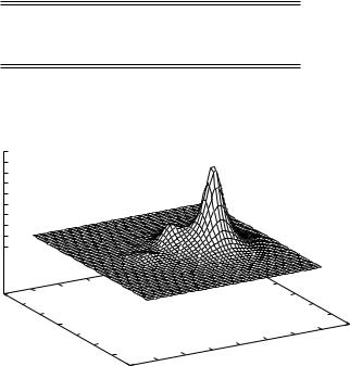
Figure 10.1. The first SCVB orbital for the allyl radical. The orbital amplitude is given in

a plane parallel to the radical and 0.5 A

distant.

and the orbitals satisfy

σyz

2 p 1

= 2 p 3 ,

(10.33)

σyz

2 p 2

= 2 p 2 ,

(10.34)

σyz

2 p 3

= 2 p 1,

(10.35)

each one consisting of a linear combination of all of the

π AOs allowed by symmetry.

In terms of HLSP functions the wave function has two terms, of course:

R

,

0.537 602 87

2 p 3

R

−

2 p 1

2 p 2

2 p 1

2 p 2

2 p 3

and the overlap between the two HLSP functions is

−0.730 003.

In Fig. 10.1 we show an altitude drawing

of the orbital amplitude

of the

first

of the SCVB orbitals of the allyl

π system. The third can be

obtained by merely

reflecting this one in the

y –z

plane of the molecule. It is seen to be concentrated at