1Foundation of Mathematical Biology / Foundation of Mathematical Biology

UCSF		Molecular similarity: 3D

3D similarity

♦Surface-based comparison approach

♦Requires dealing with molecular flexibility and alignment

♦Much slower, but fast enough for practical use

What is the algorithm?

♦Take a sampling of the conformations of molecules A and B

♦For each conformation, optimize the conformation and alignment of the other molecule to maximize S

♦Report the average S for all optimizations

Key issues: not number of atoms. Number of rotatable bonds, alignment

N	N	N	N
		O
N	N	N	N
1.00	0.97	00..9393	00..9191
N	N	N	N
N	N		N
	N	N	O

0.90	0.89		00..8888	00..8787
N	N		N	O
			O	O
N	N
		O	N	N+

HO

0.87

0.83

00..8282

00..6363

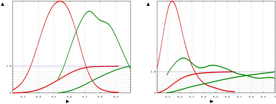
UCSF		Distributions for the two methods are very different:
		What are the quantitative overlaps?
		Molecule pairs observed crystallographically to bind the sameme sitessites
		Molecule pairs observed crystallographically to bind differentent sitessites

			Morphological Similarity				Daylight Tanimoto Similarity
(Probability distribution and integration)				(Probability distribution and integration)
	Morphological similarity					Topological similarityy

The unrelated pairs distributions are nearly normal

The related pairs distributions are multi-modal, possibly a mixture of normals

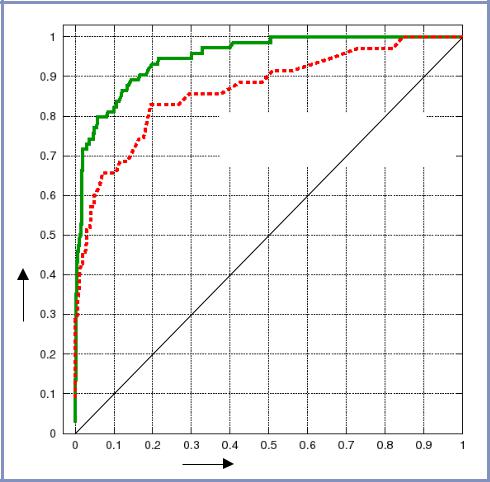
UCSF		Receiver operator characteristic curves (ROC curves)
		plot the relationship of TP rate and FP rate

To construct a ROC curve:

♦Vary the similarity threshold over all observed values

♦At each threshold, compute the proportion of true positives and the proportion of false positives

♦At low thresholds, we should have high FP, but perfect TP

♦At high thresholds, we should have low FP, but poorer TP

At a false positive rate of 0.05, MS yields a 47% reduction in the number of related pairs that are lost

At a true positive rate of 0.70, MS yields a 7-fold better elimination of false positives

Morphological Similarity

Daylight Tanimoto Similarity

True positive rate

False positive rate

UCSF		Paired data

Spearman’s rank correlation test

♦We have (Xi,Yi) for n samples

♦We want to know if there is a relationship between the paired samples, but we don’t know if it should be linear, so we need an alternative to Pearson’s r

♦Replace the (Xi,Yi) with (Rank(Xi),Rank(Yi))

♦Compute Pearson’s r for the new values

♦Alternative formulation, where d = difference in ranks for each

data pair		∑d 2
	r =1−
	s	n(n2	−1)

UCSF		Example: Spearman’s rank correlation

UCSF		Paired data

Kendall’s Tau: another rank correlation test

♦We have (Xi,Yi) for n samples

♦Definition

•Look at all pairs (Xi,Xj) and corresponding (Yi,Yj)

•Score a 1 for a concordant event

•Score a -1 for a discordant event

•Score 0 for ties in values

•Normalize result based on the number of comparisons

•We get a statistic from -1 to 1

♦Kendall’s Tau has a slightly nicer frequency distribution

♦It can be less sensitive to single outliers

UCSF

Codelet to compute Kendall’s Tau (generalized for real-valued ties)

double k_tau(double *actual, double *predicted, int n, double delta1, double delta2)

{

long int i,j;

double total = 0.0, compare = 0.0;

for (i = 0; i < n; ++i) { for (j = i+1; j < n; ++j) {

compare += 1.0;

/* first check if either is equal --> get no benefit */ if (fabs(actual[i]-actual[j]) <= delta1) {

continue;

}

if (fabs(predicted[i]-predicted[j]) <= delta2) { continue;

}

/* now check if they are correct or incorrect */

if ((actual[i] > actual[j]) && (predicted[i] > predicted[j])) total += 1.0;

else if ((actual[i] < actual[j]) && (predicted[i] < predicted[j])) total += 1.0;

else total += -1.0; /* we have a missed rank match */

}

}

if (compare == 0.0) return(0.0); return(total/compare);

}

UCSF		Paired data

Signed rank test (Wilcoxon)

♦We have (Xi,Yi) for n samples

♦Definition

•Compute all differences (Xi-Yi)

•Sort them, low to high, based on absolute value

•Assign ranks to each

•Multiple each rank associated with a negative difference by -1

•Sum the negative ranks and positive ranks

•Take the smaller magnitude sum: This is your statistic

♦Again, tables are available for small n

♦An approximation is available for large n

UCSF		Conclusions: Non-parametric statistics

Non-parametric statistics reduce reliance on distributional assumptions about your data

♦They often give very sensitive tests

♦Generally though, the corresponding parametric tests are more sensitive when it their assumptions hold

♦Note that the process is generally the same

•Compute your statistic

•Look up a significance value or compute one from an approximation

Resampling and permutation-based methods move toward deriving everything from the data observed

UCSF

BP-203: Foundations of Mathematical Biology

Statistics Lecture III: October 30, 2001, 2pm

Instructor: Ajay N. Jain, PhD

Email: [e-mail]

Copyright © 2001

All Rights Reserved