Broadband Packet Switching Technologies

SINGLE-STAGE KNOCKOUT SWITCH

147

Fig. 6.5 Ža. The 2 2 contention switch. Žb. States of the 2 2 contention switch.

having a latency of at most one bit. Note that priority is given to the cell on the left input to the 2 2 switch element. To avoid this, the switch element can be designed so that it alternates between selecting the left and right inputs as winners when there is a cell arriving on both inputs in the same time slot. However, suppose the priority structure of the 2 2 switch element were maintained and Žas described below. the concentrator were designed so that one input, say the Nth, always received the lowest priority for exiting a concentrator output. The cell loss probability for this worst case input, as N ™ , is given by

Ly1	k ey
Prwcell loss for the worst case inputx s 1 y Ý		.	Ž6.4.
ks0	k!

The above equation is obtained by considering there are k cells destined to the same output port from the first N y 1 inputs, where

Pk s žN yk	1 /ž			/k ž1 y			/Ny1yk	, k s 0, 1, . . . , N y 1. Ž6.5.
		N y	1		N y	1
As N ™ , Pk s Ž k ey .rk!. Cells at the								Nth input will be transmitted

to the output if the number of cells from the first N y 1 inputs destined for the same output port is less than or equal to L y 1. The entire summation in Ž6.4. is the probability that the cell from the Nth input will not be lost. Comparing the results of Ž6.4. with the cell loss probability averaged over all inputs, as given by Ž6.3. and shown in Figure 6.4Žb., it is found that the worst case cell loss probability is about a factor of 10 greater than the average. This greater cell loss probability, however, can be easily compensated for by adding an additional output to the concentrator.

148 KNOCKOUT-BASED SWITCHES

Fig. 6.6 An eight-input to four-output concentrator. Ž 1987 IEEE..

Figure 6.6 shows the design of an eight-input four-output concentrator composed of these simple 2 2 switch elements and single-input, single-out- put 1-bit delay elements Žmarked D.. At the input to the concentrator Župper left side of Figure 6.6., the N outputs from the cell filters are paired and enter a row of Nr2 switch elements. One may view this first stage of switching as the first round of a tournament with N players, where the winner of each match emerges from the left side of the 2 2 switch element and the loser emerges from the right side. The Nr2 winners from the first round advance to the second round, where they compete in pairs as before, using a row of Nr4 switch elements. The winners in the second round advance to the third round, and this continues until two compete for the championship: that is, the right to exit the first output of the concentrator. Note that if there is at least one cell arriving on an input to the concentrator, a cell will exit the first output of the concentrator.

A tournament with only a single tree-structured competition leading to a single winner is sometimes referred to as a single-knockout tournament: lose

SINGLE-STAGE KNOCKOUT SWITCH

149

one match and you are knocked out of the tournament. In a double-knockout tournament, the N y 1 losers from the first section of competition compete in a second section, which produces a second-place finisher Ži.e., a second output for the concentrator. and N y 2 losers. As Figure 6.6 illustrates, the losers from the first section can begin competing in the second section before the competition is finished in the first. Whenever there are an odd number of players in a round, one player must wait and compete in a later round in the section. In the concentrator, a simple delay element serves this function.

For a concentrator with N inputs and L outputs, there are L sections of competition, one for each output. A cell entering the concentrator is given L opportunities to exit through a concentrator output. In other words, a cell losing L times is knocked out of the competition and is discarded by the concentrator. In all cases, however, some cells are lost only if more than L cells arrive in any one time slot. As we have seen, for L G 8, this is a low-probability event.

For N L, each section of the concentrator contains approximately N switch elements for a total concentrator complexity of 16 NLgates. For N s 32 and L s 8, this corresponds to a relatively modest 4000 gates. Once a concentrator microcircuit is fabricated, Figure 6.7 illustrates how several identical chips can be interconnected to form a larger concentrator. The loss probability performance of the two-stage concentrator is the same as for the single-stage concentrator. In general, a K JL-input, L-output concentrator can be formed by interconnecting J q 1 rows of KL-to-L concentrator chips in a treelike structure, with the ith row Žcounting from the bottom. containing K iy1 chips. For the example illustrated in Figure 6.7, L s 8, K s 4, and J s 2.

Fig. 6.7 The 128-to-8 concentrator constructed from 32-to-8 concentrator chips.

150 KNOCKOUT-BASED SWITCHES

Fig. 6.8 Illustration of channel grouping principle.

6.2 CHANNEL GROUPING PRINCIPLE

The construction of a two-stage modular network is mostly based on the channel grouping principle w24x to separate the second stage from the first stage. With a group of outputs treated identically in the first stage, a cell destined for an output of this group can be routed to any output of the group before being forwarded to the desired output in the second stage. For instance, as shown in Figure 6.8, a cell at the top input destined for output 6 appears at the second input of the second group, while another input cell destined for output 0 appears at the first input of the first group. The first-stage network routes cells to proper output groups, and the second-stage network further routes cells to proper output ports. This smooths the problem of output contentions and thus achieves better performance complexity tradeoff for the first stage switch. More theoretical evaluations are provided as follows.

6.2.1 Maximum Throughput

This subsection focuses on the switch structure shown in Figure 6.9. An output group consists of M output ports and corresponds to an output address for the first-stage network. A cell can access any of the M corresponding output ports of the first-stage network. In any given time slot, at

CHANNEL GROUPING PRINCIPLE

151

Fig. 6.9 An asymmetric switch with line expansion ratio KMrN.

most M cells can be cleared from a particular output group, one cell on each output port.

The maximum throughput of an input-buffered switch is limited by head- of-line blocking. The symmetric case is evaluated in w8x, and the maximum throughput is 0.586. A similar approach could be taken for the asymmetric case to a point where the solution could be found by numerical analysis w20x.

Table 6.1 lists the maximum throughput per input for various values of M and KrN w20x. The column in which KrN s 1 corresponds to the special cases studied in w8x and w23x. For a given M, the maximum throughput increases with KrN because the load on each output group decreases with increasing KrN. For a given KrN, the maximum throughput increases with M because each output group has more output ports for clearing cells.

Table 6.2 lists the maximum throughput as a function of the line expansion ratio Žthe ratio of the number of output ports to the number of input ports., KMrN. Notice that for a given line expansion ratio, the maximum throughput increases with M. Channel grouping has a stronger effect on throughput for smaller KMrN than for larger KMrN. This is because for large KMrN, and

TABLE 6.1 Maximum Throughput with KrN Kept Constant While K, N ™

						Maximum Throughput
M	KrN s	1			1	1	1	1	2	4	8	16
			16		8	4	2
1		0.061			0.117	0.219	0.382	0.586	0.764	0.877	0.938	0.969
2		0.121			0.233	0.426	0.686	0.885	0.966	0.991	0.998	0.999
4		0.241			0.457	0.768	0.959	0.996	1.000	1.000	1.000
8		0.476			0.831	0.991	1.000	1.000
16		0.878			0.999	1.000

152 KNOCKOUT-BASED SWITCHES

TABLE 6.2 Maximum Throughput with KMrN Kept Constant While KM, N ™

			Maximum Throughput
M	KMrN s	1	2	4	8	16	32
1		0.586	0.764	0.877	0.938	0.969	0.984
2		0.686	0.885	0.966	0.991	0.998	0.999
4		0.768	0.959	0.996	1.000	1.000	1.000
8		0.831	0.991	1.000
16		0.878	0.999
32		0.912	1.000
64		0.937
128		0.955
256		0.968
512		0.978
1024		0.984

M s 1, the line expansion has already alleviated much of the throughput limitation due to head-of-line blocking.

6.2.2 Generalized Knockout Principle

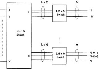
This section generalizes the knockout concentration loss calculation to a group of outputs w7, 3x. Consider an N N switch with two-stage routing networks, as shown in Figure 6.10. A group of M outputs at the second stage share LM routing links from the first-stage network. The probability that an input cell is destined for this group of outputs is simply M rN. If only up to LM cells are allowed to pass through to the group of outputs, where L is

Fig. 6.10 An N N switch with group expansion ratio L.

CHANNEL GROUPING PRINCIPLE

153

called group expansion ratio, then

1

N

N

M

k

M

Nyk

Prwcell lossx s

Ý

Ž k y LM .

1 y

.

Ž6.6.

ž k /ž

/

ž

/

M ksLMq1

N

N

As N ™ ,

L

LM Ž M . k eyM

Ž M . L M eyM

Prwcell lossx s ž1 y

/ ž1 y kÝs0

/ q

.

Ž6.7.

k!

Ž LM . !

The derivation of the above equation can be found in the appendix of this chapter ŽSec. 6.5..

As an example, we set M s 16 and plot in Figure 6.11 the cell loss probability Ž6.7. as a function of LM under various loads. Note that LM s 33 is large enough to keep the cell loss probability below 10y6 for a 90% load. In contrast, if the group outputs had been treated individually, the value of LM would have been 128 Ž8 16. for the same cell loss performance. The advantage from grouping outputs is shown in Figure 6.12 as the group expansion ratio L vs. a practical range of M under different cell loss criteria. For a cell loss probability of 10y8 , note that L decreases rapidly from 8 to less than 2.5 for group sizes M larger than 16; a similar trend is evident for other cell loss probabilities.

Fig. 6.11 Cell loss probability when using the generalized knockout principle.

154 KNOCKOUT-BASED SWITCHES

Fig. 6.12 Ratio of the number of simultaneous cells accepted to group size for various cell loss probabilities.

6.3 A TWO-STAGE MULTICAST OUTPUT-BUFFERED ATM SWITCH

6.3.1 Two-Stage Configuration

Figure 6.13 shows a two-stage structure of the multicast output buffered ATM switch ŽMOBAS. that adopts the generalized knockout principle described above. As a result, the complexity of interconnection wires and building elements can be reduced significantly, almost one order of magnitude w3x.The switch consists of input port controllers ŽIPCs., multicast grouping networks ŽMGN1, MGN2., multicast translation tables ŽMTTs., and output port controllers ŽOPCs.. The IPCs terminate incoming cells, look up necessary information in translation tables, and attach the information Že.g.,multicast patterns and priority bits. to the front of the cells so that cells can be properly routed in the MGNs. The MGNs replicate multicast cells based on their multicast patterns and send one copy to each output group. The MTTs facilitate the multicast cell routing in the MGN2. The OPCs temporarily store multiple arriving cells destined for that output port in an output buffer, generate multiple copies for multicast cells with a cell duplicator ŽCD., assign a new virtual channel identifier ŽVCI. obtained from a translation table to each copy, convert the internal cell format to the standardized ATM cell format, and finally send the cells to the next switching node or the final destination.

A TWO-STAGE MULTICAST OUTPUT-BUFFERED ATM SWITCH

155

Fig. 6.13 The architecture of a multicast output buffered ATM switch. Ž 1995 IEEE..

Let us first consider the unicast situation. As shown in Figure 6.13, every M output ports are bundled in a group, and there are a total of K groups Ž K s NrM . for a switch size of N inputs and N outputs. Due to cell contention, L1 M routing links are provided to each group of M output ports. If there are more than L1 M cells in one cell time slot destined for the same output group, the excess cells will be discarded and lost. However, we can engineer L1 Žor called group expansion ratio. so that the probability of cell loss due to the competition for the L1 M links is lower than that due to the buffer overflow at the output port or bit errors occurring in the cell header. The performance study in Section 6.2.2 shows that the larger the M is, the smaller L1 needs to be to achieve the same cell loss probability. For instance, for a group size of one output port, which is the case in the second stage ŽMGN2., L2 needs to be at least 12 to have a cell loss probability of 10y10 . But for a group size of 32 output ports, which is the case in the first stage ŽMGN1., L1 just needs to be 2 to have the same cell loss probability. Cells from input ports are properly routed in MGN1 to one of the K groups; they are then further routed to a proper output port through the MGN2. Up to L2 cells can arrive simultaneously at each output port. An output buffer is used to store these cells and send out one cell in each cell time slot. Cells

156 KNOCKOUT-BASED SWITCHES

that originate from the same traffic source can be arbitrarily routed onto any of the L1 M routing links, and their cell sequence is still retained.

Now let us consider a multicast situation where a cell is replicated into multiple copies in MGN1, MGN2, or both, and these copies are sent to multiple outputs. Figure 6.14 shows an example to illustrate how a cell is replicated in the MGNs and duplicated in the CD. Suppose a cell arrives at an input port i and is to be multicast to four output ports: 1, M, M q 1, and N. The cell is first broadcast to all K groups in MGN1, but only groups, 1, 2, and K accept the cell. Note that only one copy of the cell will appear in each group, and the replicated cell can appear at any of the L1 M links. The copy of the cell at the output of group 1 is again replicated into two copies at MGN2. In total four replicated cells are created after MGN2. When each replicated cell arrives at the OPC, it can be further duplicated into multiple copies by the CD as needed. Each duplicated copy at the OPC is updated with a new VCI obtained from a translation table at the OPC before it is sent to the network. For instance, two copies are generated at output port 1, and three copies at output port M q 1. The reason for using the CD is to reduce the output port buffer size by storing only one copy of the multicast cell at each output port instead of storing multiple copies that are generated from the same traffic source and multicast to multiple virtual circuits on an output port. Also note that since there are no buffers in either MGN1 or MGN2, the

Fig. 6.14 An example of replicating cells for a multicast connectionin the MOBAS. Ž 1995 IEEE..